Don’t hesitate to contact us:
Forum: discuss.graphhopper.com
Email: support@graphhopper.com
The latest release 0.9.0 has a new “landmark algorithm”. We introduced it as a new, third option and called it “hybrid mode” as it combines the advantages of the flexible and the speed mode. The initial algorithm was implemented fast but the implementation details got very tricky at the end and so this took several months before we could include this feature in a release.
Let us introduce you to the old routing “modes” of the GraphHopper routing engine first, before we explain the meaning and details of the new landmark algorithm.
The GraphHopper routing engine comes with the Dijkstra algorithm exploring a road network, where every junction is a node and roads connecting the junctions are the edges in the mathematical graph model. The Dijkstra algorithm has nice properties like being optimal fast for what it does and most importantly being able to change requirements per request. So if you want to route from A to B and you want to avoid motorways or tolls or both you can easily change these requirements per request. There are also the faster, still optimal bidirectional or goal directed variants. The speed up there is approx. 4 times. Note that this speed-up is often very similar to the explored nodes in the graph and so here we do a comparison of the different algorithms based on the visited nodes via a ~130km example route:
Unidirectional Dijkstra with 500K visited nodes
Bidirectional Dijkstra with 220K visited nodes
Unidirectional A* with 50K visited nodes
Bidirectional A* with ~25K visited nodes
Note that GraphHopper is able to change the cost function used to calculate the best path on the fly, e.g. you can change the shortest or fastest path per request. This cost function is called the “weighting” internally which is independent of the calculation used for the time of the route.
The problem with Dijkstra and also A* is that these algorithms are still too slow for most real world graphs. GraphHopper does its best and serves responses for A* in roughly a second on average even for longer country wide routes, but tuning it lower than this is hard if you want to keep flexibility and optimality. And routing through a continent or several countries is only reasonably doable if you tune your algorithm to special use cases or if you sacrifice optimality. Even with current hardware.
Researchers of the KIT have invented many nice routing algorithms and one of them was “Contraction Hierarchies” (CH), which is still a bidirectional Dijkstra but works on a “shortcut graph” giving response times of under 100ms for routes across a whole continent. Some researchers might be nitpicking and say we have a slow implementation but probably they measure response times for just the distance calculation. Here we are talking about the full route calculation, with getting the instructions and geometry (without latency) in under 100ms and of course this is much faster for country-wide queries.
The visited nodes picture looks very sparse:
Contraction Hierarchies with ~600 visited nodes
The newly developed landmark algorithm is an algorithm using A* with a new heuristic based on landmarks and the triangle inequality for the goal direction. Note that despite using this heuristic the algorithm still returns optimal routes. Also, this algorithm was developed earlier than CH so only “new” in GraphHopper.
For this algorithm we need a few landmarks that indicate where the graph “looks” beneficial to explore. A landmark can be any node of the graph and to make the algorithm work we have to calculate distances from these landmarks to all nodes of the graph. So assume the following graph, where the number between the nodes is the distance (“edge weight”) and node 1 and 4 are our two landmarks:
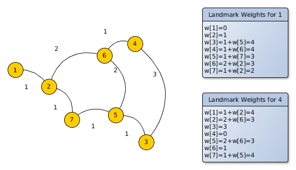
The tables on the right show the distances for the two landmarks to all the other nodes. For example the pre-calculated weight for landmark “node 1” from node 2 is 1km, from node 3 it is 4km and so on. The same for the landmark “node 4”: the weight from node 1 is 4km, from node 2 it is 3km and so on. This means if you want to route from node 3 to the landmark “node 4” you already know the best weight, which is 3km or from node 3 to the landmark “node 1” it is 4km. But how would you use these landmark weights for arbitrary queries? The idea is to use A* which requires a weight approximation and you normally get the approximation w(XD) to the destination D via beeline estimates, now in this algorithm the triangle inequality is used. The only requirement is that this weight should not be overestimated:
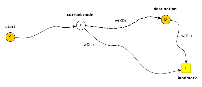
w(XD) + w(DL) >= w(XL)
w(XD) >= w(XL) – w(DL)
In real world we can pre-calculate w(DL) for all landmarks. The rest of the implementation is a bit more complex as the graph is directed and you have more landmarks, and other stuff that we’ll highlight later on. The good news is that we are allowed to pick the maximum of all calculated values for the different landmarks.
Here it is important to highlight the limitation of this algorithm compared to the flexible mode: without recalculating the landmark weight tables we can only increase an edge weight. If we would do a decrease the resulting routes could be suboptimal. But for most scenarios this works nicely (traffic jams make your weights higher) or you can invert the requirement to make the rest slower. Furthermore for all the other scenarios where this is not possible or to complex a recalculation of the landmark weights is fast even in the world wide case and can be made parallel.
To pick the best landmarks we are not using a completely random algorithm, which would be fast but we would get no real speedup. Instead we pick only the first node at random, then search the farthest node which is our first landmark. Then start from this landmark 1 to search again the farthest node being our landmark 2. And now we put these two landmarks as start in our graph search to search landmark 3 which is farthest from 1 and 2. And so on. This results in landmarks at the boundary of our graph and roughly equally spread, which is exactly what we need.
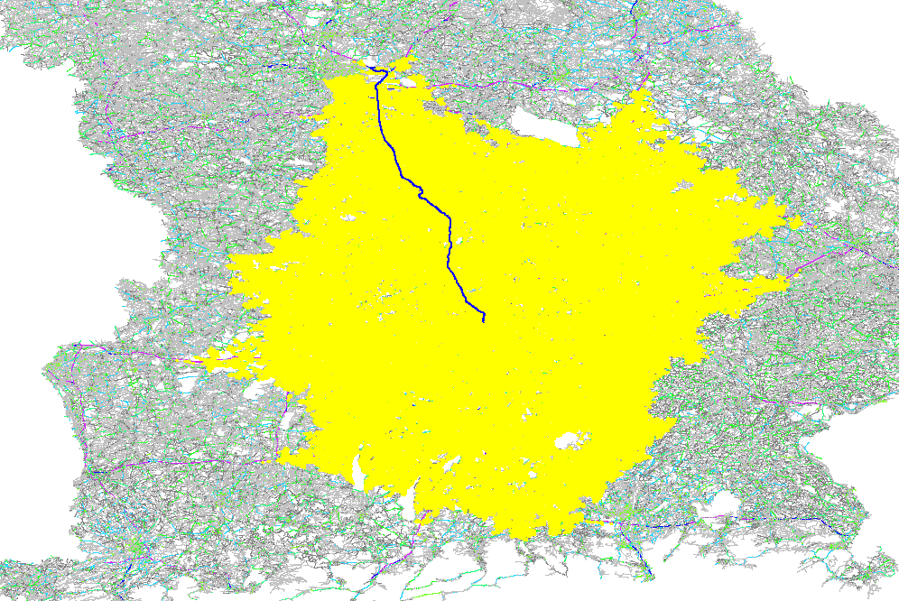
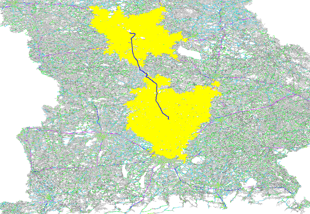
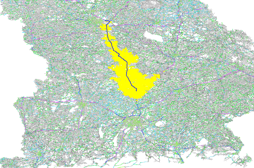
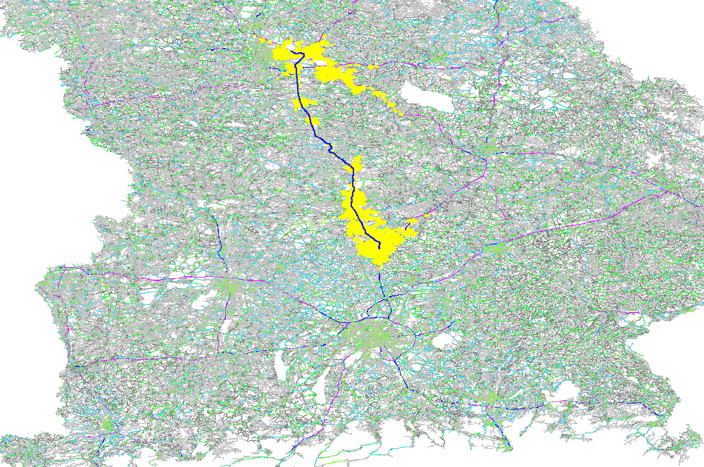
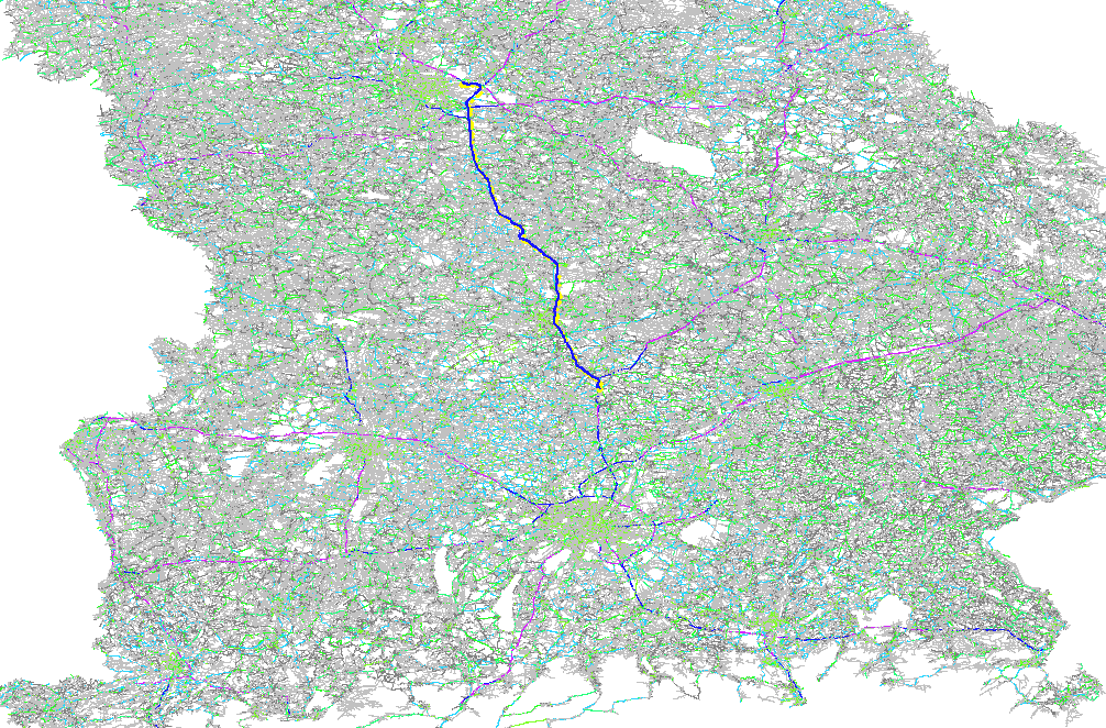
This search can be independent on the used weighting. We initially started with shortest and it works mostly, but for bigger continental scale it was producing strange clustered landmarks leading to slower results compared to handpicked landmarks. So what we really wanted is not a ‘farthest’ in terms of geometry but ‘farthest’ in terms of the density or topology of the graph. I.e. an equal distance between the nodes and so a simple breadth-first search resulted in the best quality. Here is an example of Bavaria a part of south Germany:
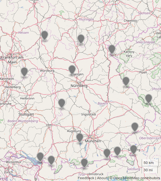
Automatic Landmark Selection for Bavaria, Germany
For every request it turns out that not all landmarks are equally usable and we pick a set of active landmarks. This could be dynamically changed but in our tests this didn’t improve the query speed consistently.
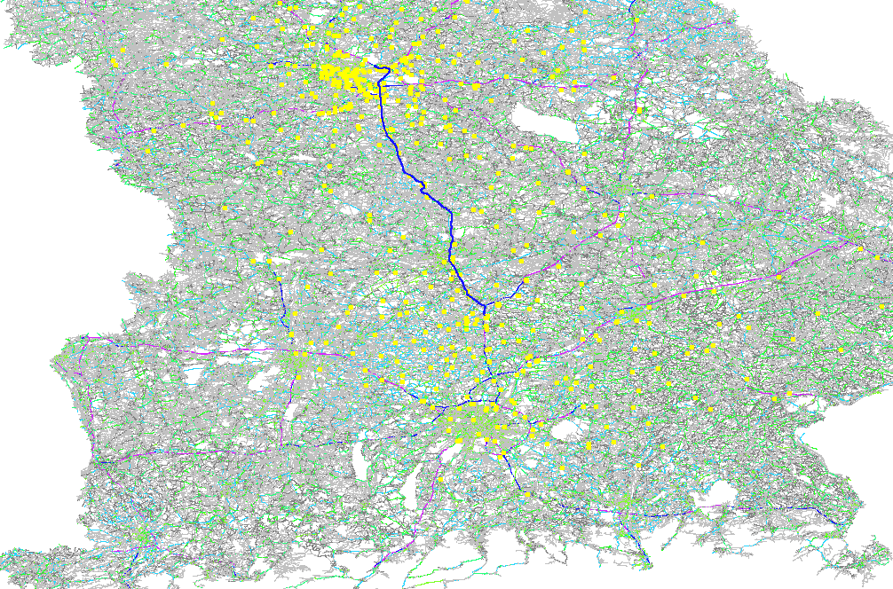
As we picked a bit extreme example route the visited nodes for the landmark algorithm look even better than that of the CH calculation, which is not the case on average:
landmark algorithm with only ~300 visited nodes
Here we’d like to highlight again that the landmark algorithm can be very efficient compared to the normal A*:
Bidirectional A* with ~25K visited nodes
As already mentioned above our underlying data structure knows only nodes that are junctions. But how would we handle a start or destination that starts somehow on an edge? We introduce so called “virtual nodes” (and virtual edges) in our graph that live only in an isolated QueryGraph for the time span of the request. With this concept the underlying algorithm does not need to know about such virtual query nodes (and edges). The problem for the approximated weights for the landmarks algorithm is that the pre-calculated values are only done for the junction nodes and we have to carefully pick the correct weight of the neighboring junction node to maintain correctness. So the approximation procedure needs to be aware of virtual nodes, which is a bit unsatisfying but seems to be necessary.
You have to calculate landmarks for every subnetwork. We had the subnetwork algorithm already there (Tarjan) and reused this algorithm. Coming to this conclusion was the trickiest conclusion, as we previously assumed a simple connectivity check would be sufficient, but real world showed it was not.
You can calculate the storage requirement as follows. A good start are 16 landmarks and lets say we use Germany. Germany has roughly 9 mio edges and we store the distance in a short (2 bytes) and this is necessary for forward and backward direction of every edge, then we need 2*2*16*9mio bytes, i.e. ~550MB just for this speedup data which is twice as large as the speedup data for CH but the 16 landmarks are created faster. Although GraphHopper supports memory mapping you should use the default “in-memory” configuration to keep everything fast. And because of this we cannot waste memory and have to make compromises on the way to achieve this, just to make it working on a global scale.
One of the compromise is to store every distance in a short. This is not easy if you have both: short edges and long ferry ways across a continent. And so we artificially disallow routing across certain borders e.g. currently only within Europe, within Africa, Russia and South-East Asia. We think this cutting is reasonable for now and are then able to store 16 landmarks in ~5GB of memory for the world wide case per precomputed vehicle profile.
The query speed for cross country are as follows where we always picked 8 as active landmarks.
| Landmarks | Average Speed/ms | Speed up compared to A* (~1.2s) |
| 16 | 72 | 17x |
| 32 | 46 | 26x |
| 64 | 33 | 36x |
For this specific test we used the OpenStreetMap data from 16.02.2017 for Germany with 8.6 mio nodes and 10.9 mio edges in the road network.
This is a really good speed improvement compared to the flexible routing with Dijkstra or A*. Still the speed of contraction hierarchies is ~10 times faster on average. The speed advantage of CH gets lost as soon as we go into a more dynamic scenario like with traffic information or blocking certain roads and also handling other scenarios where we consider the heading of a vehicle are straightforward to implement with the landmarks algorithm but complex with CH.
The downsides of this new ‘hybrid mode’ compared to the flexible mode are that it requires substantially more memory and changing edge weights has to be done carefully. Furthermore if you force the algorithm to take completely different routes than the best ones, e.g. with a per-request requirement to avoid a whole country, then the performance degrades to the one of A*.
