Don’t hesitate to contact us:
Forum: discuss.graphhopper.com
Email: support@graphhopper.com
OpenStreetMap (OSM) is a free digital map of the world that is created and maintained by millions of users. Among many other things it includes detailed information about every possible type of road, ranging from narrow hiking trails in the mountains to the biggest motorways. Using the open source GraphHopper routing engine you can easily turn this data into a calculator that tells you the optimal route between a start and target location.
GraphHopper features a fast and memory-efficient import of the currently over 200 million OSM ways and answers routing queries within milliseconds even for continental length. One of the main benefits of doing this yourself is that you can fully customize the route calculations according to your specific use case, be it the next hiking app or delivery management system.
In this blog post you will learn how to set up and use the GraphHopper server. There are a few trade-offs you should know about and this article will give you an idea how you can make the most out of it with the resources you have available.
The first thing you need is of course a recent version of GraphHopper. Since it is written in Java you also need a recent JVM (Java 8 or newer) and obviously you need some OSM data to import. Let’s start with a small map like the one of Berlin – i.e. download the PBF file.
All of the important GraphHopper configuration is written in a configuration file config.yml:
graphhopper:

  datareader.file: berlin-latest.osm.pbf
  graph.location: berlin-gh
  profiles:
    - name: bike
      vehicle: bike
      weighting: custom
      custom_model_file: empty
    - name: foot
      vehicle: foot
      weighting: custom
      custom_model_file: empty
    - name: car
      vehicle: car
      weighting: custom
      custom_model_file: empty
      turn_costs: true
      u_turn_costs: 60

server:
  application_connectors:
  - type: http
    port: 8989
    bind_host: localhost # for security reasons bind to localhost
  request_log:
      appenders: []
As you can see, it points to the OSM PBF file, defines a folder called berlin-gh that GraphHopper will create and use to store all its data, and three different ‘profiles’ that use the default settings for traveling by bike, foot or car. The configuration also specifies that the server will be available at port 8989. Take a look at the example configuration to learn more about these and many other configuration options.
You can now start the service using the following command:java -jar graphhopper-web-[version].jar server config.yml
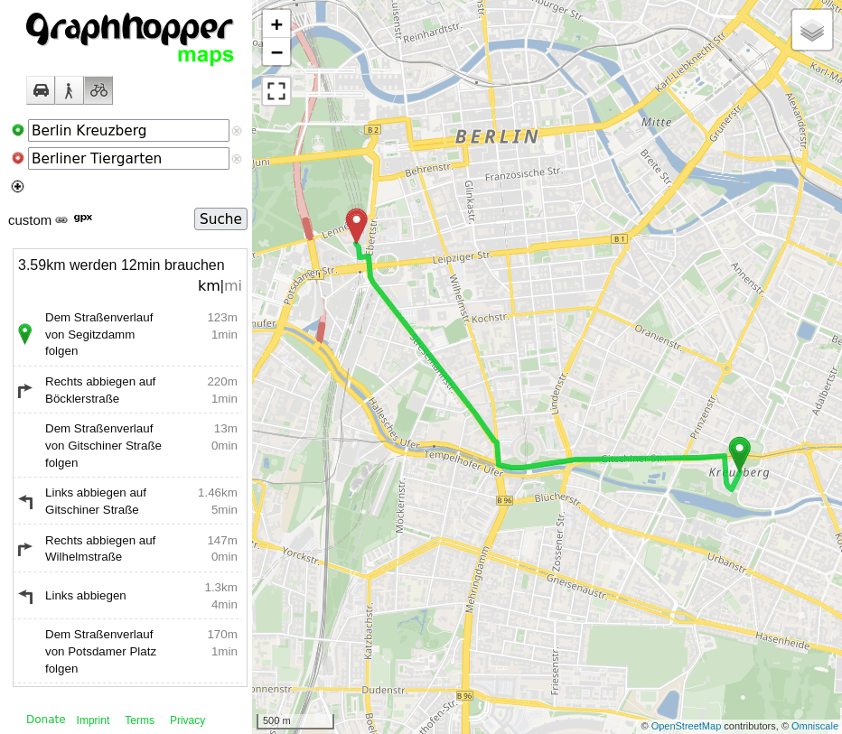
Within a few seconds this will load the OSM file, run the data import, store everything in the berlin-gh folder and start the server. You should now be able to see the GraphHopper Maps UI in your browser under http://localhost:8989/maps and query the GraphHopper server’s REST API under http://localhost:8989/route. The next time you run this command GraphHopper will load everything from the berlin-gh folder, so you will no longer need the OSM file and the import won’t run again.
When it comes to customizing the routing calculations the most important part is the possibility to create different profiles, which specify routing-related properties like the speed used for different road types. While they are written in the server configuration they can be modified to a certain extent for every single routing request. You can change e.g. the speed used on motorways for the car profile or exclude steps for the foot profile when requesting a route.
The following custom model avoids primary and high speed roads for the bike profile:
{
 "priority": [{
   "if": "road_class == PRIMARY",
   "multiply_by": 0.1
 }, {
   "if": "max_speed >= 50",
   "multiply_by": 0.1
 }]
}
The syntax is explained in detail here. Note that the best way to tweak your custom model is to use the interactive custom model input box of the GraphHopper Maps UI. Once you are happy with your custom model you can copy it to a file named bike.json and reference it in the bike profile of your config.yml file like this:
graphhopper:
  ...
  profiles:
    - name: bike
      vehicle: bike
      weighting: custom
      custom_model_file: bike.json
This way the customization will become the default for queries using the bike profile and still you can adjust it further from the client side. Note that when you make changes to your routing profiles you need to run the import again. So either delete the berlin-gh folder or change the graph.location and use another folder.
In the previous section only the OSM data was imported to build what we call the ‘base graph’, i.e. the road network graph that is used for the route calculations. This is all you need for route calculations, but one of GraphHopper’s most prominent features is that it is able to do this much faster (multiple orders of magnitude). For this it uses a special algorithm called Contraction Hierarchies (CH) which we also sometimes refer to as ‘speed mode’. The faster query speed may not be so relevant for small maps like the Berlin example map, but really does make a difference for larger maps as you will see in a moment. Enabling CH is as simple as adding the following lines to your configuration file:
graphhopper:
  # ... same as above
  profiles_ch:
    - profile: bike
    - profile: foot

  prepare.ch.threads: 2
This enables CH for the bike and foot profiles (but not for car). When you execute the server command as above, GraphHopper will run the CH preparation and store additional data in the berlin-gh folder unless it is there already. Otherwise it will load it from the same folder. The setting prepare.ch.threads allows you to run multiple CH preparations in parallel, which speeds up the process, but requires more memory. Note that the profiles you use CH for can of course use your own custom model files, like bike.json in the above example, which means you can first tweak your custom model and then speed up the routing using CH.
For certain use cases that only require a rough estimate of the time and distance between two locations GraphHopper allows for another performance improvement: You can disable turn restrictions by setting turn_costs: false in the configuration and benefit from a less demanding CH preparation (e.g. for worldwide setup it takes ~3h instead of ~25h and much less memory) and you will also get faster query response times (roughly 1.5-2x faster).
While CH is very fast it has one major drawback: Since it uses index data that is specific for the profiles written in the server configuration, the routing profiles cannot be changed on a per-request basis. Therefore, GraphHopper supports another great algorithm, the so-called Landmarks algorithm (LM), which offers slower queries than CH, but is still a lot faster than normal Dijkstra or A* and allows for adjustments of the routing profile per-request. You can enable it in a very similar way as CH by adding the following lines to the config file:
graphhopper:
  # ... same as above
  profiles_lm:
    - profile: bike
    - profile: foot

  prepare.lm.threads: 2
There is one important restriction for LM when you want to change the custom model at runtime: The weights used for each road can only be increased, but never decreased. So for example increasing speeds or priorities is prohibited but they can be decreased at will. An easy workaround is using large speeds in your server profile, but keep in mind that the routing queries will be the faster the closer the adjusted speeds are to the ones that were used when running the LM preparation.
Of course you can add LM and CH profiles for the same profile at the same time. When CH is available it will be the default, but you can still use the ch.disable=true parameter to make use of LM. And if LM is available you can disable it using lm.disable=true to gain full flexibility.
Until now you learned how GraphHopper deals with a small OSM data set for the city of Berlin. However, from the very beginning it was one of GraphHopper’s primary goals to handle the full planet file, which nowadays contains over 60GB compressed geographic information of the world. Handling this amount of data in a fast and memory-efficient way is a real challenge and one thing where GraphHopper shines. By the way, this part is even utilized in planetiler – the (fastest?) tool to create planet-scale vector tiles from OSM data.
So let’s talk about how to use GraphHopper for larger maps and what to do in a few common situations.
Continental sized maps or even the full planet file require a lot more memory and initial processing time. Both are roughly proportional to the size of the map, which can either be approximated directly by the size of the OSM file or expressed by the number of ‘edges’ (connections between road junctions) of the GraphHopper graph. Take a look at the following table, created using the above configuration (without CH):
| Map | OSM PBF size in GB | number of edges in millions |
| Berlin | 0.07 | 0.5 |
| Bayern (Germany’s biggest state) | 0.7 | 4.7 |
| Germany | 3.6 | 24.3 |
| North America | 12 | 89.7 |
| Europe | 25 | 147.0 |
| Planet | 64 | 415.9 |
The first thing you need to do when using larger maps is increasing Java’s heap size. This is done using the Xmx flag, e.g.java -Xmx4g -jar graphhopper-web-[version].jar import config.yml
will set the heap size to 4GB. If you set this value too small the import can become very slow or even fail due to insufficient heap memory. In this case you will usually an exception thrown by the JVM, but be aware that in some cases also the operating system might kill the process. How large the heap space needs to be depends on the size of the map and a few more choices you can make.
Also note that here we used the import command rather than the server command as we did previously. This is always recommended when running imports for larger maps. Compared to the server command the import command does not start the server when the import is complete, but in turn it is able to free up memory that is no longer needed during the import process. When the import is done you can just use the server command with the same configuration to start the server.
For lowest possible latency of routing requests you should also enable a low latency garbage collector (GC) for the JVM (Note that for the import command this is not recommended). In our experience a low latency GC is important not only for very large heaps but already when the Xmx setting is above 5GB. We use ZGC in production since several years (enable it via -XX:+UseZGC) and another good choice can be Shenandoah GC (-XX:+UseShenandoahGC).
For an updated deployment guide please see our documentation.
At the time of this writing (May 2022) and with the short configuration from the top and this change:
graphhopper:
  ...
  profiles_ch:
    - profile: car
    - profile: bike

  prepare.ch.threads: 1 # more threads require even more memory
you can start the import with:
java -Xmx120g -Xms120g -jar graphhopper-web-[version].jar import config.yml
Without the option -Xms the JVM always tries to reduce its heap size (to release it to the operating system) which might result in a busier garbage collector that you should avoid.
Likely, these memory requirements sound extraordinary to you. Please keep in mind that in this case GraphHopper holds the road network of the entire world in memory plus the “speed up” data. Compared to other open source routing engines with the same fast query speed, the memory requirements of GraphHopper are still lower as you can run one instance with multiple profiles (the road network data is shared). Furthermore, GraphHopper still offers you “per-request” flexibility as you can deactivate the CH algorithm for each individual requests. See the next section.
At the time of this writing (May 2022) and with the short configuration from the top and this change:
graphhopper:
  ...
  profiles_lm:
    - profile: car
    - profile: bike

  prepare.lm.threads: 1
you can start the import command:
java -Xmx60g -Xms60g -jar graphhopper-web-[version].jar import config.yml
As previously explained, LM requires less time than CH when turn_costs are enabled and still allows for flexible routing queries.
| configuration | base graph | import time | preparation size | preparation time |
| car+bike+foot no CH, no LM | 33GB | 1h | – | – |
| car+bike+foot CH: car + bike | 33GB | 1h | 27.5GB for car 8GB for bike | 25h for car 3h for bike |
| car+bike+foot LM: car + bike | 33GB | 1h | 20GB for car 19GB for bike | 3.5h for car 3.5h for bike |
The CH and LM preparations are meant to speed up the routing queries at the cost of a longer import time and more memory usage. If your hardware does not provide enough memory the easiest thing you can do is just not use these speed-up techniques at all. Even without these GraphHopper is still fast, especially for shorter routes. In this case you might want to enforce a maximum query distance to prevent long running routing requests and make sure you do not run out of memory at query time. This is done using the setting routing.non_ch.max_waypoint_distance: 1000000
which limits the maximum query distance to 1000km for example. You can also have a look into routing.max_visited_nodes. There are a few more ways to reduce the memory needed to start the GraphHopper server:
GraphHopper is very efficient when it comes to using the same road network for multiple routing profiles. For example if you use different profiles for various types of cars, trucks and motorcycles there will be only a small increase of the required memory, because a lot of data will be shared between these different profiles. However, there are certain roads that aren’t used by certain vehicles at all. For example the foot profile might never use motorways, or a car profile might never use foot- or cycleways. GraphHopper ignores unused roads entirely, so you can reduce the size of the graph by separating profiles that use different sets of road types. Especially separating motorized vehicles from non-motorized ones (like bike and foot) can make a big difference. It won’t reduce the overall memory requirement, but you might be able to use two smaller machines instead of a single big one.
You can also configure GraphHopper such that it does not load the imported graph into memory at all. This way you can drastically reduce the memory requirement, but the import will be much slower. For example importing the planet file will take about three days rather than about 1.5 hours. To enable memory mapping you need to set graph.dataaccess.default_type: MMAP
in the config file. When using MMAP you should try to use a maximum of 50% of the physical memory for Xmx. This way there is enough heap space for objects created during the import and the operating system has enough memory for the memory mapped graph data.
Another advantage of using MMAP compared to RAM_STORE is that it speeds up the server startup time as less data is loaded initially. The query speed will be slower, though. If you want to still preload the data into memory you can since v5.0.
Importing OSM data requires more memory than actually running the server using the imported data. Therefore you can use a larger machine with more memory to run the import command and then copy the GraphHopper folder to one or more smaller machines where you start the server using the server command.
Note that you can also use a combination of MMAP and RAM_STORE. If you use different hardware for the import and the routing service it can help to use MMAP only for the routing service. This way you can benefit from a fast import and smaller memory requirements on your routing server.
This blog post gives you an overview of how you can run GraphHopper under real world circumstances. It describes the most common settings to adapt it to your needs and mentions some important performance tweaks that are especially useful for large maps, like the import command and the MMAP setting which can help in memory constrained situations.
With GraphHopper you can stay flexible and use ordinary server hardware even when you load worldwide OSM data. And when you need to scale the request volume you can enable a speed boost with a special algorithm called Contraction Hierarchies or Landmarks. All with just a tiny configuration change.
This combination of flexibility and fast queries is one of GraphHopper’s biggest strengths.
Get involved and if you have questions about this topic feel free to ask them in our forum!
