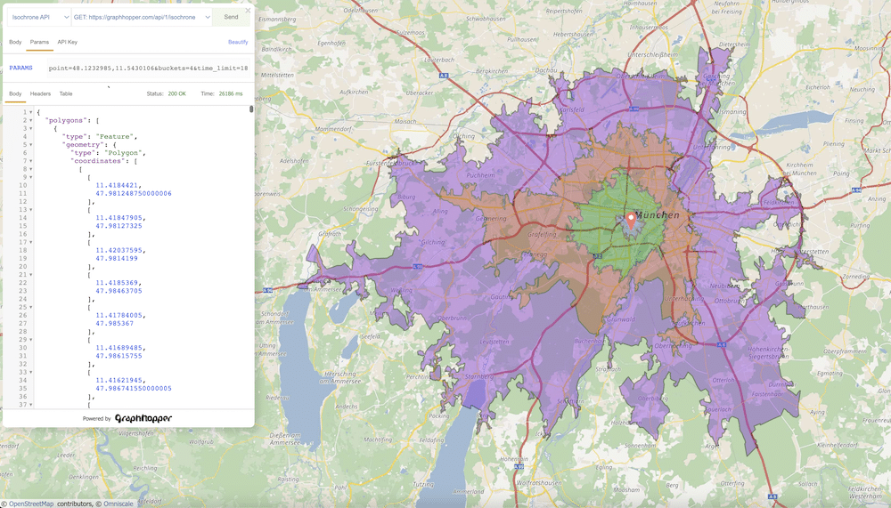
Here is a little preview of our latest development, our API Explorer. It’s not just an ordinary tool to examine API requests & responses in a JSON editor. Our API Explorer comes with a unique feature that will make your development process a lot more fun: a map at the center of it all!

With our API Explorer, you can now easily visualize the result of your requests on a map. In the attached picture, you can see the result of a request to our Isochrone API. We’ve queried which areas can be reached from our headquarters in Munich within a 30-minute car ride, and the map shows the answer.

We can’t wait for you to try it out and see how it can take your development process to the next level. Stay tuned for more updates!

We have released the next version of GraphHopper, the flexible and fast open source routing engine for OpenStreetMap. Read more about it on GitHub and read on to find out what’s new.

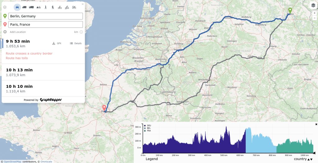
When you start the new GraphHopper Routing Engine, you will be greeted by the new GraphHopper Maps. We have blogged about it earlier and you can try it out at graphhopper.com/maps:

One long awaited feature is that GraphHopper can now handle also more complex turn restrictions (by @easbar and @lukasalexanderweber). The most common cases for turn restrictions were already well supported, but sometimes the current turn restriction depends on the previous road from which one reached the current road and this required special handling. This was rather tricky to implement and improves routing for e.g. navigation applications, especially in larger cities where such restrictions may occur more frequently:

In the new GraphHopper version you can now easier store the OSM way IDs (by easbar). This improves the interaction with other applications like a PostgresSQL/PostGIS database or similar where you store your own properties per way ID from OpenStreetMap and want to enhance e.g. the GraphHopper response with these properties.

Customizable Routing

There are now new EncodedValues like “curvature” and “footway”. E.g. with “curvature” you can create custom models that prefer curvy roads or avoid them which can be quite powerful in combination with the “urban_density” or slope related EncodedValue released in the previous version.

We improved the response speed for heavier customized profiles and the hike profile has now more realistic times.

Changes to Areas

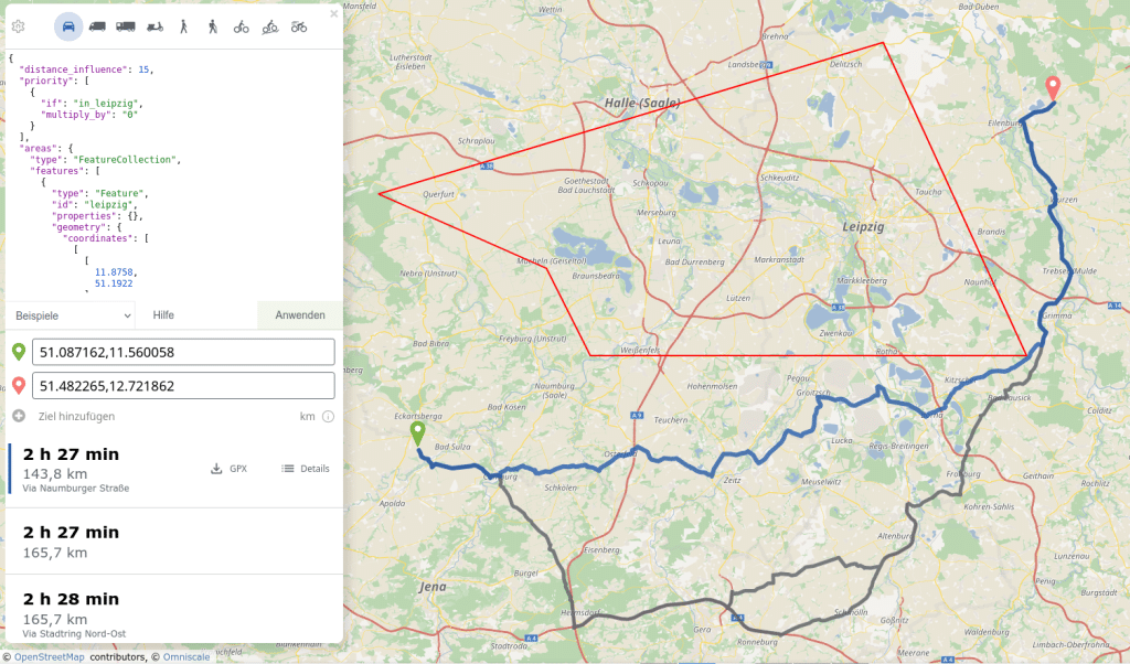
You can now also define custom areas outside of a custom model, so that you can create multiple models without creating the same areas again. We now use the FeatureCollection as format in the custom model to make it easier to use with other tools. And you can see the areas directly in GraphHopper Maps:

Contributors

Thanks a lot to all contributors!

easbar, boldtrn, michaz, lukasalexanderweber, otbutz, karussell, ratrun, OlafFlebbeBosch

Many Other Bug Fixes and Improvements

• Improve instructions for U-turns by @easbar
• The country geometries are more precise by @karussell
• The custom weighting is now the default by @karussell
• Avoid hills in a custom model by @karussell
• New intersections path detail by @boldtrn
• Remove YAML support for server-side custom models by @karussell
• Improve area check precision by @otbutz
• Consider bicycle routes if tagged with “lcn=yes” by @ratrun
• Support “;” access delimiter for bikes by @ratrun
• Replace com.wdtinc MVT library with no.ecc by @easbar
• Use explicit ignore list for highway values by @easbar
• Maxspeed fix by @karussell
• contributing nb_NO and updating pl_PL by @OlafFlebbeBosch + this.
• i18n: updated sv_SE by @OlafFlebbeBosch
• Split vehicle tag parsers into access, speed and priority by @easbar and @karussell
• Use multi-threading for subnetwork preparation by @easbar
• Make sure waypoints are not removed during path simplification by @easbar
• … and many more
• See also the changelog for potential breaking changes

Start using GraphHopper

You can see the new version in action on graphhopper.com/maps, or install it locally on your laptop or server. Do not hesitate to ask questions or leave feedback in our forum.

Happy routing!

We are constantly working to improve our software to better serve our customers. We solve millions of vehicle routing problems every day. Over 90% of these problems are actually variations of the famous traveling salesman problem, which requires finding the shortest possible route that visits all the locations exactly once. As we see these problems being solved in the mobile context more often, just like ordinary shortest path problems (from an origin to a destination), we also see the need to solve these problems faster and faster. We are excited to announce our latest performance improvement: we can now solve traveling salesman problems up to 50% faster!

To solve real world Traveling Salesman problems, we essentially need to solve 2 main sub-problems which have to be solved one after the other: the shortest path problem to calculate all travel times and distances between all locations and the actual Traveling Salesman problem to determine the best sequence of these locations.

We have already written a detailed article about our incredible fast Matrix API and how we solve the first subproblem, i.e. the shortest path problem. It can be read here. The improvements made on the second subproblem can be summarized as follows:

Firstly, we have optimized our software and hardware to take even more advantage of parallel processing, which means that we can now solve multiple parts of the problem simultaneously (on hardware that is suited best for these kind of tasks). This has dramatically reduced the time required to find a solution.

In addition, we have developed new heuristics that enable us to quickly eliminate non-optimal routes and focus on the most promising paths. This helps us to converge on a solution more quickly and with greater accuracy.

These enhancements enable us to solve traveling salesman problems as quickly as it is illustrated in the following figure. The traveling salesman problems used here are typical last mile delivery problems with random stops in Munich.

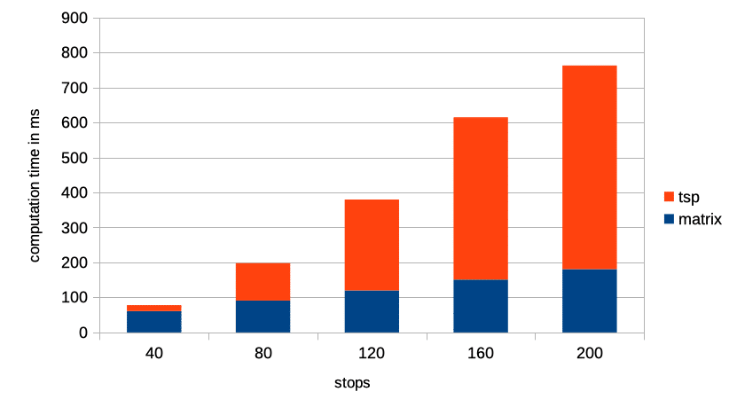
The figure shows the computation times in milliseconds (y-axis) for 5 traveling salesman problems varying in size (x-axis). The travel times are calculated based on OpenStreetMap. Furthermore, it differentiates between the computation time of the matrix (all travel times and distances between all locations, e.g. 40×40 or 120×120 travel times) and of the traveling salesman problem (tsp). As you can see, a traveling salesman problem with 120 stops can now be solved in 380ms. The matrix takes 120ms and searching for the best sequence 260ms*.

It takes slightly more time if you solve these traveling salesman problems with (day)time-dependent travel times from TomTom. To solve this type of problem, we compute multiple matrices to account for traffic and peak and off-peak travel times (see here for an article describing how we derive time-dependent travel times).

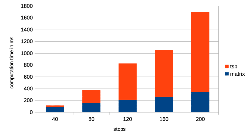
As illustrated in the figure above a traveling salesman problem with 120 stops takes 825ms in total (209ms for the matrix, 616ms for the sequence)*.

These improvements mean that our customers now get faster results enabling them to optimize their operations more effectively. At the same time, we – for our part – can solve these problems even more efficiently and thus more problems with the same computing capacity, which in turn allows us to offer our service at attractive prices.

We are committed to continuously improving our software and providing our customers with the best possible service and are excited to see the impact our latest performance improvement will have on our customers’ businesses. If you have any questions or would like to learn more about our software, please don’t hesitate to get in touch. If you are new to GraphHopper and just want to try our service without contacting us and without any further obligations, you are welcome to register here. Then you will get a free Standard plan for two weeks.

Happy Routing!

Your GraphHopper Team

*_{All computation times shown above are average numbers (from 100 runs). The traveling salesman problems are solved on our fastest dedicated setup, i.e. if you register here to try out our service, it takes slightly more time.}