Findings on Route Optimization in Practice – Part 1

When we founded & started the GraphHopper company in 2016, we had quite a decent theoretical knowledge about vehicle routing problems and solution methods to solve these problems. With our Route Optimization API it was possible to solve different traveling salesman problems at that time. The simplest traveling salesman problem can be explained as follows: The task is to visit a number of places exactly once and to find a round trip between these places, i.e. we start our tour at one place and gradually visit all other places exactly once and return to our starting point. This tour should be as efficient as possible, i.e. for example as fast as possible or as short as possible, or to put it more generally, it should minimize my cost function.

We had at that point, the somewhat naive notion that minimizing a transport cost function consisting of a linear combination of total time and distance is probably quite sufficient. Our customers will be happy to have a tool at their fingertips to determine the order of places to visit so that these costs are as low as possible. Needless to say, we thought the solutions we came up with were fantastic.
However, feedback from some of our customers painted a slightly different picture. The tours we calculated may have been theoretically nice in the sense of a round trip that minimizes the cost function we thought is sufficient. In practice, however, some drivers found that our tours were sometimes a bit too cumbersome – sometimes even a bit annoying – and not exactly intuitive. I.e. these drivers seem to want to take into account not only time and distance, but other costs and preferences unknown to us at that time.
In other words, what we have learned is that in practice minimizing that transport cost function may be a pretty decent approximation, but in no way can we assume that we know all the components of the driver’s or our customer’s cost function with it.

To make this a little more tangible, I’d like to write further about a driver preference that we have encountered again and again. To give a very simple example, we have often made route proposals of the following type:

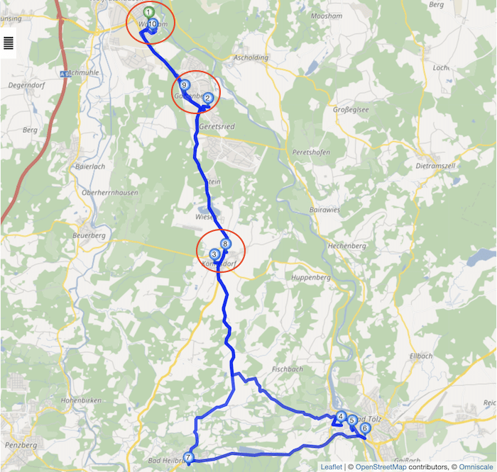
This is the solution that solely minimizes our transport costs. The numbers on the blue marker indicate the stop sequence. The green marker shows the start and end location of the vehicle. What can be very annoying from the driver’s point of view is that he has to return to an area where he has stopped before (red circles, i.e. stop 1 and 10, 2 and 9, 3 and 8).
While our computers only know nodes, edges and costs, the driver very likely sees many small for the driver consistent and self-contained delivery areas. And if the driver delivers in a certain area at the beginning, then he definitely does not want to return to this area at the end of his tour to deliver packages to a few more customers. This may have something to do with costs that are unknown to us but theoretically quantifiable, e.g. parking search costs, but it may also be that he simply perceives the tour as bad – even if the tour is by no means bad with regard to the objective criteria known to us.

We see several ways to account for that in our solution approach. First, we can identify these many small delivery areas beforehand and then schedule accordingly contiguously, i.e. the stops in a delivery area are always scheduled one after the other. Second, we can modify our cost function to accommodate this preference. We have been successfully experimenting with both approaches. What is most promising for us at the moment is to adjust the cost function & solution search so that stops are processed as early as possible. That is, we have added to our cost function the preference to deliver to customers as early as possible. So, if there are a number of more or less equivalent solutions with respect to the above transport cost function, we now prefer solutions in which all customers are supplied as soon as possible. This leads to better consideration of the discussed driver preference, i.e. it is generally avoided that drivers have to approach certain areas twice.
If I solve the example problem from above again today with our service, I get the following route:

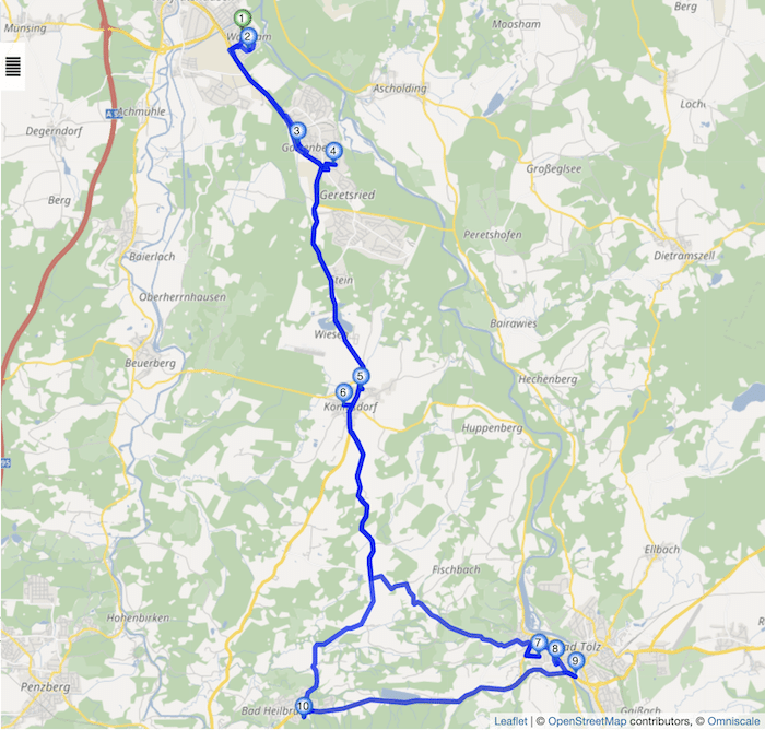
For many of our customers, this has allowed us to significantly improve our route suggestions. Therefore, I can justifiably write that this improvement has led to greater acceptance of our routes and, as a result, happier customers. But, of course, we also learned that this is very dependent on the underlying vehicle routing problem. For example, if the transported weight is a significant cost factor, the solution is of course dependent on the activity at the customer’s site, i.e. whether goods are unloaded or loaded. Thus this is just one example of what we have learned and used from our customers. I will write down more examples in the future.

If you want to solve your own traveling salesman problems and if you are not a GraphHopper user yet, get a free API key or check out our open source projects on GitHub.

Have fun optimizing your routes!