In this blog post we’ll describe how custom profiles can be used and include real world examples.

How to

You can try the examples on GraphHopper Maps. Please note that currently only for car, small_truck, scooter, bike and foot the custom routing support is deployed. To customize a request you click on the “custom” icon. When editing the custom model try out Ctrl+Space for auto complete e.g. inside an if-statement. The basic structure of a custom profile is described in this documentation.

Safe Biking

Let’s start with a simple example from the previous post – it shows how to avoid primary roads:

{
 "priority": [{
   "if": "road_class == PRIMARY",
   "multiply_by": "0.1"
 }]
}

Other possibilities are for example to avoid roads with higher speed signs and prefer official bike network:

{
 "priority": [{
   "if": "max_speed >= 50",
   "multiply_by": "0.1"
 }, {
   "if": "bike_network == MISSING",
   "multiply_by": "0.9"
 }]
}

Avoid tunnels:

{
 "priority": [{
   "if": "road_environment == TUNNEL",
   "multiply_by": "0.01"
 }]
}

Ride slower through e.g. pedestrian or footway. Here 5 minutes instead of 4:

{
 "speed": [{
   "if": "road_class == PEDESTRIAN",
   "multiply_by": "0.7"
 }]
}

Cargo Bike

The normal bike profile allows routing over steps in cases where otherwise a long detour is made. But a bike used for deliveries or children cannot be carried and should never be routed over this and so you can exclude it with the road_class encoded value:

{
 "priority": [{
   "if": "road_class == STEPS",
   "multiply_by": "0"
 }]
}

Further exclusions like ‘too narrow roads’ are possible which is important for e.g. cargo bikes:

{
 "priority": [{
   "if": "max_width < 1.5",
   "multiply_by": "0"
 }, {
   "if": "road_class == PRIMARY",
   "multiply_by": "0.1"
 }]
}

Walking for Tourists

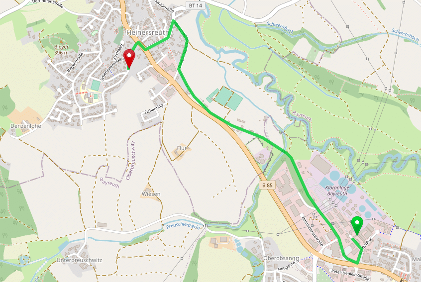
Increase preference of the official hiking network and accept greater detours. As you can see in the custom profile all roads marked with “foot_network=other” are avoided and so e.g. “foot_network=regional” is used.

{
 "priority": [{
   "if": "foot_network == MISSING",
   "multiply_by": "0.5"
 }]
}

Economically Driving

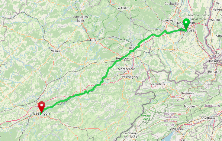
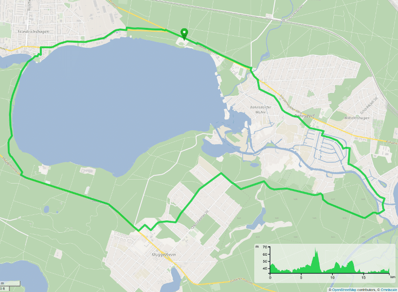
There are many ways to save fuel. One is to drive slower and another is to prefer shorter routes. See how the custom profiles can look:

{
 "speed": [{
   "if": "true",
   "limit_to": "110"
 }],
 "priority": [{
   "if": "road_class == MOTORWAY || road_class == SECONDARY",
   "multiply_by": "0.4"
 }]
}

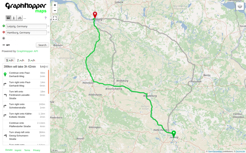
Prefer shorter routes. Here the faster motorway is avoided. To do that you increase the distance_influence:

{
 "distance_influence": 200
}

The distance_influence is independent of the road properties and does not influence the ETA. The default is 70 in seconds per 1km. Let’s assume a route that takes 1000sec and is 10km long, then a value of 30 means that I would like to drive maximum 11km to reduce the travel time to 970sec, or drive max 12km to reduce it to 940sec.

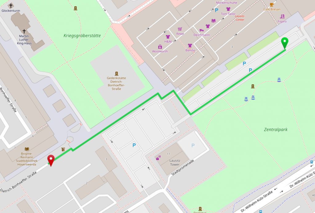
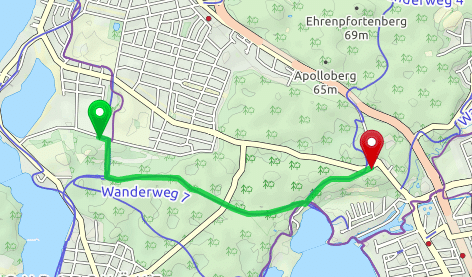
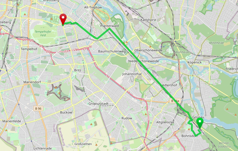
Now to the area feature:

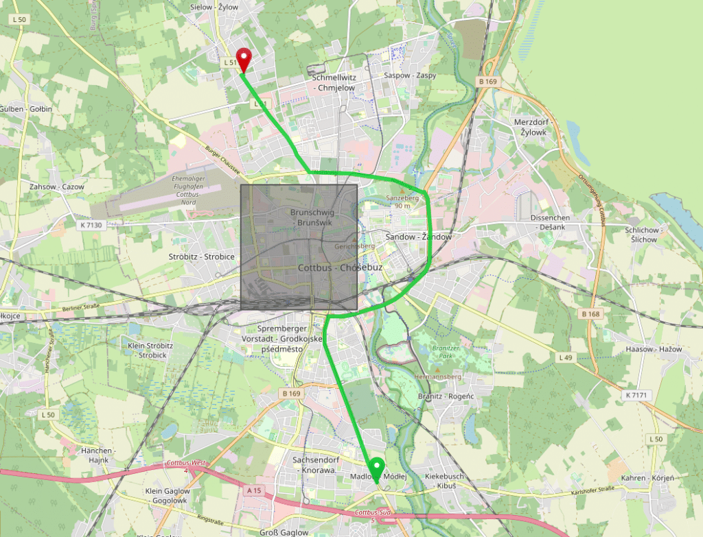
Click on the image to calculate the route and paste the following profile:

{
 "priority": [{
   "if": "in_cottbus",
   "multiply_by": "0"
 }],
 "areas": {
   "cottbus": {
    "type": "Feature", 
    "properties": {},
    "geometry": { 
      "type": "Polygon", 
      "coordinates": [[
       [ 14.31, 51.75 ],
       [ 14.34, 51.75 ],
       [ 14.34, 51.77 ],
       [ 14.31, 51.77 ],
       [ 14.31, 51.75 ]
      ]]
    }
   }
 }
}

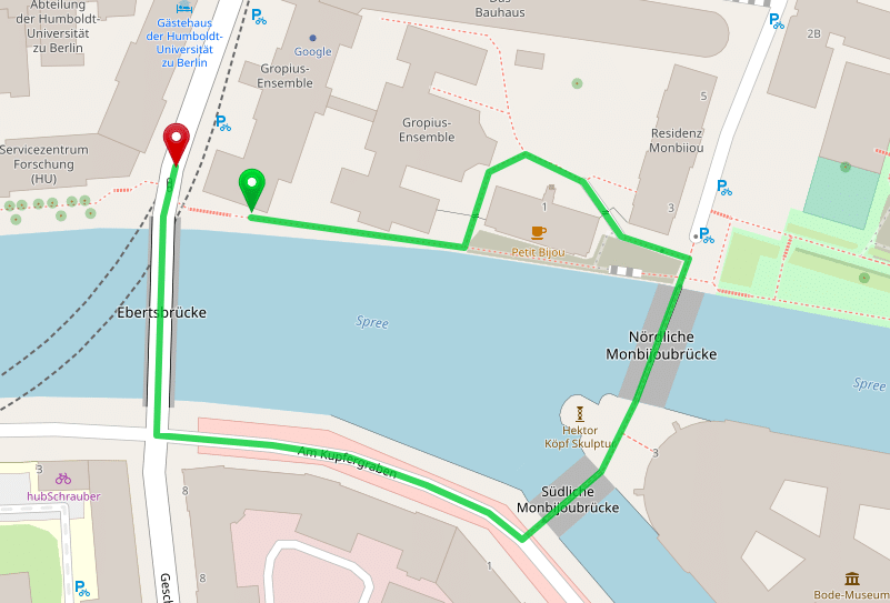
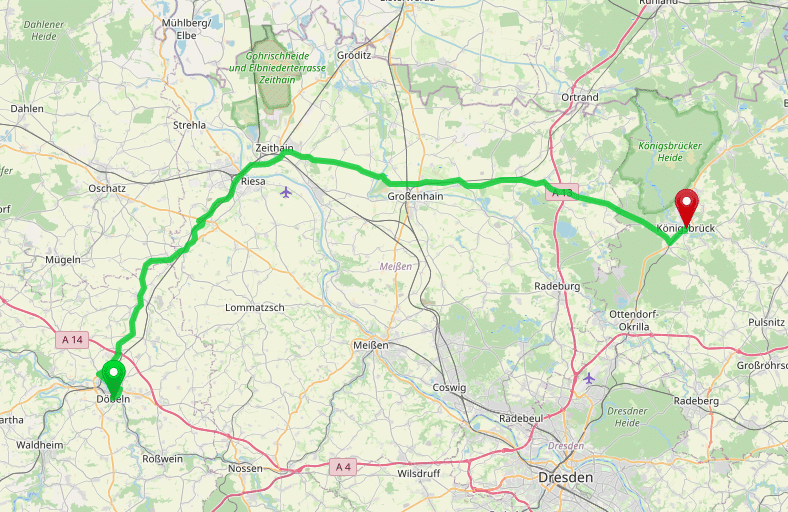
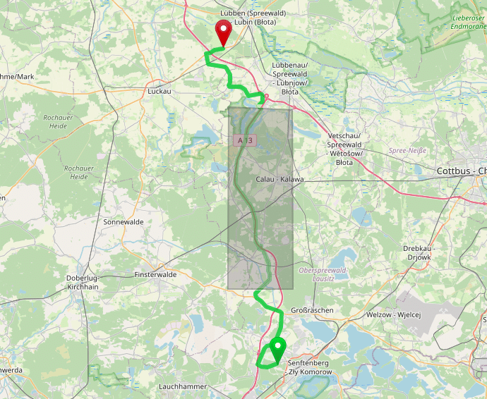
A powerful concept is to combine areas with arbitrary other conditions. E.g. you can prefer or avoid certain roads only in or outside of an area. The following example avoids the motorway only outside of the specified area:

{
 "priority": [{
   "if": "road_class == MOTORWAY && in_near_calau == false",
   "multiply_by": "0"
 }],
 "areas": {
  "near_calau": {
    "type": "Feature",
    "properties": {},
    "geometry": {
      "type": "Polygon",
      "coordinates": [[
        [ 13.84826, 51.6137 ],
        [ 13.9746, 51.61375 ],
        [ 13.97323, 51.82983 ],
        [ 13.84963, 51.83323 ],
        [ 13.84826, 51.6137 ]
      ]]
    }
   }
 }
}

Truck

You can use custom profiles to give the car profile several “truck” attributes. First of all you should reduce the max_speed and the speed and increase the distance_influence like we did for the “economically driving”.

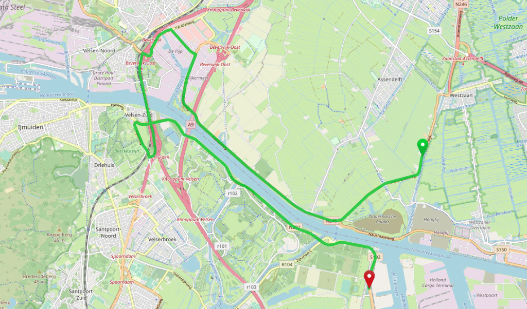
Further changes can be done like avoiding ferries:

{
 "priority": [{
   "if": "road_environment == FERRY",
   "multiply_by": "0.1"
 }, {
   "else_if": "road_class == RESIDENTIAL || road_class == TERTIARY",
   "multiply_by": "0.3"
 }, {
   "else_if": "road_class == TRACK",
   "multiply_by": "0"
 }]
}

Now to the typical truck use cases like avoid toll, width or height limitations:

{
 "priority": [{
   "if": "toll == ALL || toll == HGV",
   "multiply_by": "0.1"
 }]
}

Consider more truck properties:

{
 "priority": [{
   "if": "hazmat == NO || hazmat_water == NO",
   "multiply_by": "0"
 }, {
   "if": "hazmat_tunnel == D || hazmat_tunnel == E",
   "multiply_by": "0"
 }, {
   "if": "max_width < 3 || max_weight < 3.5 || max_height < 4",
   "multiply_by": "0"
 }]
}

Conclusion

As already mentioned this feature will strongly benefit from your feedback. So do not hesitate to share your experience, custom profiles or problems you are running into!

Happy custom routing!

Today, after more than 8 years of work, we are releasing version 1.0 of the open source GraphHopper routing engine.

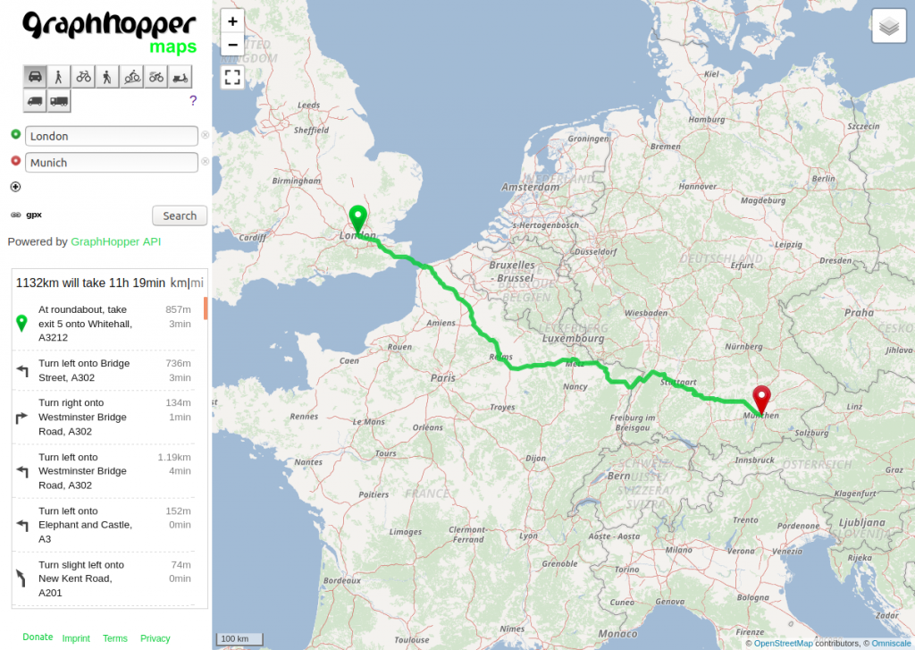
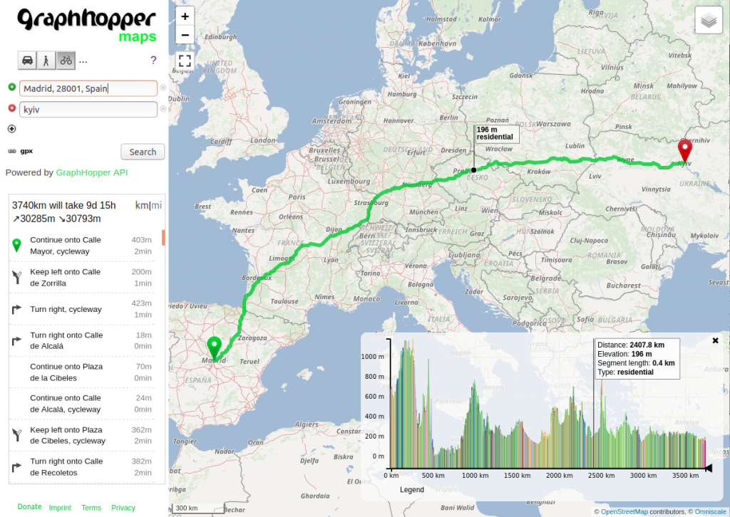
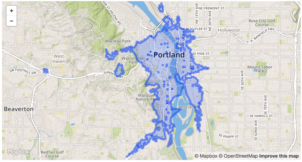
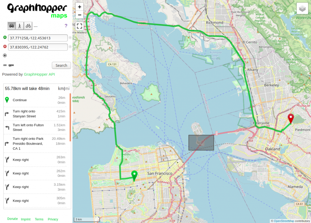
GraphHopper calculates optimal routes in road networks (for example taken from OpenStreetMap) for many different vehicle types and finds the ideal itinerary when using public transit. It is released under the Apache License 2.0 and you can easily try its road routing capabilities on GraphHopper Maps. Besides the route calculations the GraphHopper engine offers a lot more features like the map matching (“snap to road”), the navigation and the isochrone calculation (for a point it finds all reachable roads within a specified time). See the end of this post for some impressions and view GraphHopper on Github!

Since the last stable release 0.13 a few months ago we merged over 115 pull requests and were able to fix over 50 issues on Github. Many contributors were involved in the new 1.0 release:

easbar, michaz, msbarry, boldtrn, karussell, oflebbe, otbutz, Janekdererste, sguill, samruston, aoles, don-philipe, ratrun, taulinger, naser13, HarelM, twitwi, Anvoker and devemux86.

Thank you!

The new features

The new features in more detail:

• Customizable routing: Without knowledge of Java and just some JSON (or YAML) configuration you can now tweak the default vehicle profiles. You can do this on a per-request basis, but also use your configuration with the fast hybrid- and speed modes. Use this to avoid bridges, motorways, ferries, steps or certain areas, avoid roads with truck limits, change the speed or max_speed variables or prioritize certain road classes like official bike routes. You can get very creative here! From @karussell and @easbar. To find out more see the documentation, issue #1841 and this blog post. Or try on this demo server and click on the flex icon near the ‘Search’ button.
• A major code refactoring that includes turn costs calculation within the ‘Weighting’ class from @easbar. See our changelog.
• A major refactoring towards profiles that replaces the ‘weighting’ and ‘vehicle’ parameters with a new ‘profile’ parameter. This requires some configuration changes. For the most cases you can use our converter tool. See the documentation. From @easbar.
• Alternative route calculations are now much faster as they benefit from node- or edge-based Contraction Hierarchies #1722 from @michaz
• Isochrone refactorings and improvements like edge-based graph traversal and turn restriction support from @michaz. See e.g. #1824.
• Add new ‘curbside’ parameter #1697 to approach roads from a specific side from @easbar.
• Bilinear interpolation for elevation #1942 from @msbarry
• Many changes and improvements for spatial rules from @otbutz
• Updates to our iOS port graphhopper-ios#47 from @oflebbe
• Several bug fixes for the Landmark algorithm from @michaz and @aoles
• a new POST /route endpoint, in addition to the GET /route endpoint, which avoids URL-length limitations, allows request compression and more from @karussell
• More encoded values like EU tunnels, hazmat (hazardous materials), etc. from @otbutz
• A new vehicle profile ‘wheelchair’ #1726 from @don-philipe
• Many bug fixes for the block_area and the country feature from @karussell
• Improvement for point hints #1935, from @samruston. This additionally improved query speed by 10%.
• A big improvement to reduce the memory requirements for the import. Mainly from @msbarry
• A new user interface for public transit from @Janekdererste and @michaz
• Improved turn instructions like #1882 (or this) from @boldtrn
• Edge-based Tarjan algorithm and subnetwork removal to avoid connection not found problems if turn restrictions are enabled (#2044) from @easbar
• A good speed improvement for path details from @easbar
• Turn instructions now give hints about ferries, tolls and private roads
• Upgrade to Dropwizard 2.0
• Several changes to reduce FlagEncoder usage.
• Start to use JUnit5 in tests from @Anvoker and @easbar
• A StringIndex allowing to store strings per edge that will allow several improvements for turn instructions in the future

The new features complement these existing features:

Happy Routing!

The upcoming version 1.0 of the GraphHopper routing engine has a new customizable routing feature.

Disclaimer: We updated the format for custom models. See the updated blog post with several examples.

To install GraphHopper with this feature on your own server download the JDK, the routing server, the configuration file and the OpenStreetMap data:

# if you have no JDK installed get it from: https://adoptopenjdk.net/
wget https://oss.sonatype.org/content/groups/public/com/graphhopper/graphhopper-web/1.0/graphhopper-web-1.0.jar
wget https://raw.githubusercontent.com/graphhopper/graphhopper/1.0/config-example.yml
wget http://download.geofabrik.de/europe/germany/berlin-latest.osm.pbf

Now edit the downloaded config-example.yml and add the following car profile, please note that indentation is important in YAML:

graphhopper:
  ...

  profiles:
    - name: car
      vehicle: car
      weighting: custom
      custom_model_file: empty

  # also add the configuration:
  routing.ch.disabling_allowed: true

Then you can start the java server:

java -Ddw.graphhopper.datareader.file=berlin-latest.osm.pbf -jar graphhopper-web-1.0.jar server config-example.yml

which should give you a similar log output:

...
 io.dropwizard.server.ServerFactory - Starting GraphHopperApplication
...
c.g.reader.osm.GraphHopperOSM - version 1.0|2020-05-01T21:00:45Z (5,15,4,3,5,6)
c.g.reader.osm.GraphHopperOSM - start creating graph from berlin-latest.osm.pbf
...
c.g.routing.ch.CHPreparationHandler - 1/1 calling CH prepare.doWork for profile 'car' NODE_BASED
...
c.g.reader.osm.GraphHopperOSM - flushing graph CH|car|RAM_STORE|2D|no_turn_cost|5,15,4,3,5, details:edges:133 725...
...
org.eclipse.jetty.server.Server - Started @23477ms

When you start the server the first time it will take a bit longer as it creates the road network (the part after “start creating graph”) and helper files (the part of CHPreparationHandler) inside the graph-cache folder.

Now open the GraphHopper Maps demo UI that is available on your local machine: http://localhost:8989/maps/?point=52.48947%2C13.346329&point=52.565917%2C13.450699&profile=car

Click on the small “flex” button near the “Search” button and a text input will open. Include the following:

priority:
  road_class: { primary: 0.5 }

to e.g. avoid primary roads (see below for “prefer”). The route will be evaluated on-the-fly and the query speed is already perfect for most real world scenarios.

Increasing the priority of primary roads works a bit different: decrease the priority of “all other roads”, which can be done using the so called “catch-all” key and set the priority of primary to 1.0:

priority:
  road_class: { primary: 1.0, "*": 0.5 }

Learn More About CustomWeighting

To learn more about the possibilities read the documentation. Also you’ll notice that when you place the cursor in the text input on e.g. “road_class” it will list all available values like motorway or footpath, or place it on “priority” this will list all available so called “encoded values” like road_class, but also road_environment (bridge, tunnel, …). By default several useful “encoded values” are already available. For example click on the top right button and select “Omniscale Dev” and “Local MVT” then you can hover your mouse and see the “encoded values” road_environment, road_class and max_speed on the left panel for every road segment:

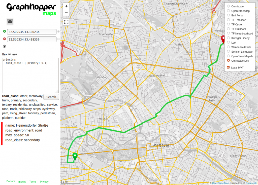
You can add more encoded values like surface or toll when you add the following in the config-example.yml:

graph.encoded_values: surface,toll,max_width,max_weight,max_height,hazmat,toll,track_type

To make them available in the graph you have to:

1. stop the server
2. remove graph-cache and
3. start the server again.

This procedure is always required when you want to make changes to the graph itself, so more or less every time you edit the config-example.yml or when you want to update the OSM data.

Fast Response Times for CustomWeighting

To have a fast response also for longer routes like across Europe you put the customization in a YAML (or JSON) file and provide this at import time. I.e. create a local file profile1.yml with the following content:

priority:
  road_class: { primary: 0.5 }

In the config-example.yml file replace:

 custom_model_file: empty

with

 custom_model_file: profile1.yml

Now again remove the graph-cache folder and restart the server again.

When you now open the UI the default vehicle profile will already avoid the primary road_class without the need to specify this in the request. But the big difference is the query speed. You won’t notice this for the Berlin example, still you try a larger area, e.g. download a OSM pbf file for a bigger area (and remove the graph-cache to force a re-import) and try this again.

Contraction Hierarchy and Landmark Preparation

Technically we enabled a Contraction Hierarchy (CH) preparation for the custom car profile, this is called the speed mode, see the profiles_ch section in config-example.yml. This step introduces shortcut edges and uses a special query to significantly improve query speed for long routes. The downside is that currently you cannot further customize a “CH prepared profile” per-request.

To get faster response times and still being able to customize the profile per-request you can enable the hybrid mode which uses the landmark (LM) preparation under the hood:

graphhopper:
  ...
  profiles_lm:
  - profile: car

To make this change available you again need to remove graph-cache and restart the server.

Get a more sophisticated profile in this truck example file.

More Playground

Let’s add a bike profile and highly prefer roads that are part of the official bike network. To do this first add the bike flag encoder and also change the profiles section:

graphhopper:
  ...
  graph.flag_encoders: car,bike

  profiles:
    - name: car
      vehicle: car
      weighting: custom
      custom_model_file: empty
    - name: bike
      vehicle: bike
      weighting: custom
      custom_model_file: empty

Remove the graph-cache folder and restart the server again. You’ll now see also bike in the logs:

c.g.reader.osm.GraphHopperOSM - using CH|car,bike|RAM_STORE|2D|no_turn_cost

When the server is ready you’ll again being able to open the previous link: http://localhost:8989/maps/?point=52.48947%2C13.346329&point=52.565917%2C13.450699&profile=car

The only tiny difference is that a bike icon is additionally displayed. Click on it. You’ll get an error which reads:

Cannot find CH preparation for the requested profile: 'bike' You can try disabling CH using ch.disable=true available CH profiles: [car]

This error tells us that we cannot use speed mode for our new bike profile yet. We have two options: 1) We can keep using the profile using the hybrid mode and further adjust it to our needs and 2) we can enable speed mode once we are fully satisfied with our settings. Let’s see how this works.

Option 1

Disable the speed mode (CH) in the request, i.e. append a special parameter to the URL which will be forwarded to the routing server: http://localhost:8989/maps/?point=52.48947%2C13.346329&point=52.565917%2C13.450699&profile=bike&ch.disable=true

This is sufficient to try out the custom weighting with bike. Click again on the “flex” icon near the “Search” button and enter the following text:

priority:
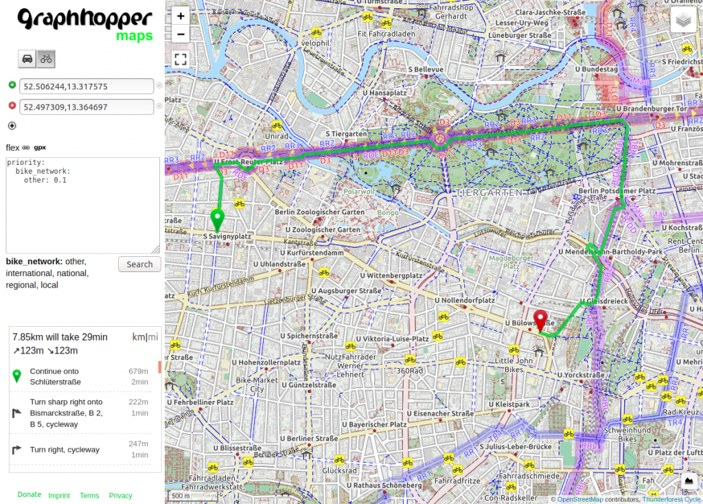
  bike_network: { other: 0.4 }

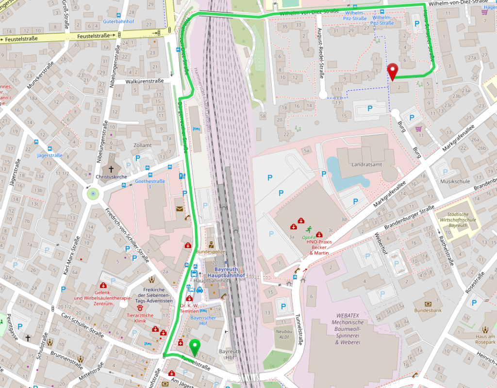
When you click again on the button in the top right corner and select “TF Cycle” some nice bike maps will appear. The blue, purple or red marked roads are official recommended routes from different bike networks. And with the steps above we avoid all roads that are not part of this network. You can reduce the number to e.g. 0.1 and see that the route will “snap” to these official bike network even if that means a huge detour:

Get a more sophisticated “cargo bike” profile in this example file.

Option 2

Now we can enable the speed mode also for bike. To do that we only have to add “bike” to the profiles_ch section in the config-example.yml:

graphhopper:
  ...
  profiles_ch:
    - profile: car
    - profile: bike

Then once again remove the graph-cache folder and restart the server again. You’ll now notice the following two entries in the logs:

c.g.routing.ch.CHPreparationHandler - 1/2 calling CH prepare.doWork for profile 'car' NODE_BASED
c.g.routing.ch.CHPreparationHandler - 2/2 calling CH prepare.doWork for profile 'bike' NODE_BASED

Which means that it will use a bit more RAM (and space on disk) but also take a bit longer. After that you’ll be able to click on the bike icon:
http://localhost:8989/maps/?point=52.48947%2C13.346329&point=52.565917%2C13.450699 or follow this link to get the bike icon pre-selected. Now with this additional “CH preparation” also the bike profile responds fast even for long-distance routes.

If you have questions or feedback for this tutorial, you can comment in this topic.