Don’t hesitate to contact us:
Forum: discuss.graphhopper.com
Email: support@graphhopper.com
This article describes how we calculate and prepare travel time matrices to solve time dependent vehicle routing problems.
Let me first explain what a typical vehicle routing problem is: Given a vehicle fleet and a number of customers, find the optimal set of vehicle routes to serve all customers and to minimize total transportation costs, e.g. the sum of vehicles’ travel times. A vehicle route is then a sequence of customers along with point-to-point routes on the legs between them.
To solve these vehicle routing problems (VRPs), we require travel times between all customer and vehicle locations. Let me assume we have n locations in total, we need to calculate a (n x n) travel time matrix. In most cases, it is more advantageous to calculate this matrix before the actual vehicle routing problem is solved rather than during the optimization.
If we need to solve VRPs with constant travel times, i.e. travel times not being dependent on departure times, we need to calculate a single (n x n) matrix. That’s it! Based on this, we can start solving the VRP.
However, travel times usually vary significantly throughout the day. Therefore, they are dependent on vehicles’ departure times. In urban areas, travel times are largely influenced by the rush hours of private traffic. Unfortunately, this implies also that there is a unique (n x n) travel time matrix for each possible departure time. To put it in other words, even if the vehicle routing problem is small, we need to calculate thousands of these (n x n) travel time matrices. This is not feasible. If we still calculated these matrices, we would often observe only minor variations between matrices, especially if departure times were very similar. Therefore, it is reasonable to split a typical day into time slices of constant travel times which reduces this arbitrary number of (n x n) matrices to the number of time slices.
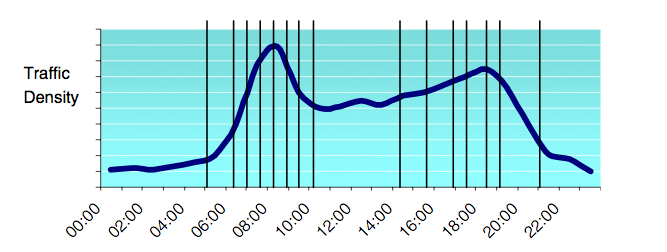
[Source: Eglese et al. (2006) – Road time table]
The figure above shows typical variations in traffic densities and travel times during a day. Furthermore, it illustrates appropriate time-slices to account for these variations. So we can calculate a (n x n) travel time matrix for each time slice. That’s it!
I am afraid, it is not yet sufficient since these slices of constant travel times yield to a discrete travel time function with leaps from one slice to another. These leaps result in an unrealistic property, i.e. vehicles with the same origin and destination can pass each other. For example, if we had two time slices: peak (7am-9am) and off-peak (9am-11am). In peak hours, it takes 2 hours to get from origin to destination, in off-peak hours it only takes 1 hour. Vehicle v1 starts in peak at 8:59 and, thus, takes 2 hours. Vehicle v2 starts only 2 minutes later at 9:01 and only takes 1 hour. Vehicle v2 passes v1 and reaches destination almost 1 hour earlier than v1. This is unrealistic and only caused by artificially slicing the day to save travel time matrix calcuations.
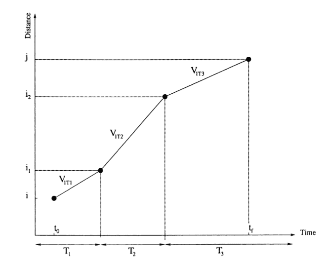
[Source: Ichoua et al. (2003) – Travel speed function]
Therefore, – as suggested in Ichoua et al. (2003) – we transformed constant travel time matrices of each time slice into constant speed matrices. This, in turn, results in a continuous travel time function. Getting back to the example above: Let me assume that the distance from origin and destination amounts to 100 km. For our peak slice, it does not take 2 hours from origin to destination, but vehicles can drive 50 km/h on this relation in the time from 7am to 9am. In off-peak hours, vehicles can drive 100 km/h on the exact same relation. This means that if a vehicle starts at 7am, it takes 2 hours for 100 km. If it starts at 8am, it takes 1 hour for the first 50 km and 1/2 hour for the second 50 km, i.e. in total it takes 1 1/2 hour. If it start at 8:59, it takes a bit longer than 1hour. Et voilà! Now we can start solving the actual time-dependent VRP.
If you are interested in even more details, if you have comments or if you want to try out our Time-Dependent Optimization API based on TomTom’s historic traffic data, please do not hesitate to contact us. If you are interested in how fast we can calculate travel time matrices for each time slice, let me recommend you this article.
Happy Routing!
References:
Richard Eglese, Will Maden, and Alan Slater. A road timetable to aid vehicle routing and scheduling. Computers and Operations Research, 33(12):3508 – 3519, 2006. ISSN 0305-0548. doi: 10.1016/j.cor.2005.03. 029. URL http://www.sciencedirect.com/science/article/pii/S0305054805001243. Part Special Issue: Recent Algorithmic Advances for Arc Routing Problems.
Soumia Ichoua, Michel Gendreau, and Jean-Yves Potvin. Vehicle dispatching with time-dependent travel times. European Journal of Operational Research, 144(2):379–396, 2003. ISSN 0377-2217. doi: 10.1016/ S0377- 2217(02)00147- 9. URL http://www.sciencedirect.com/science/article/pii/S0377221702001479.
Load balancing in the context of vehicle routing problems is a way to achieve a more evenly distribution of jobs or activities over your drivers’ routes. There are a number of reasons to balance load. The most obvious ones are resource utilization and fairness.
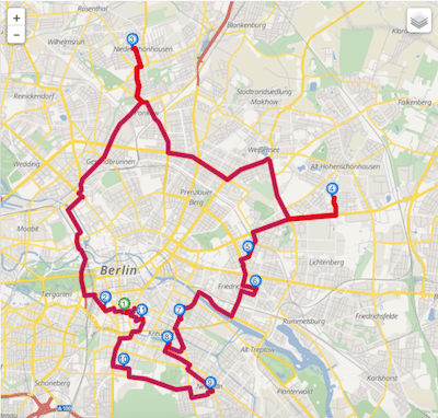
Simply because there are a number of optimization goals and in many cases planners want to minimize vehicles and variable transportation costs. However, this is often contrary to balanced vehicle routes. Let us illustrate this with a simple example. Assume there are four drivers with the same start location (green marker). They need to conduct 10 deliveries (blue marker). There are no further constraints like capacity restrictions or time windows. If your first optimization goal was the minimization of vehicles, and, the second, the minimization of completion times, you would specify it as follows:
{ "objectives": [
   { "type": "min", "value": "vehicles" },
   { "type": "min", "value": "completion_time" }
  ]
}
The best solution is to just deploy a single vehicle as illustrated in the figure below.
To achieve this, you need to refine the optimization goal. GraphHopper offers you three simple ways:
When using this goal, GraphHopper minimizes the maximum of completion time of all employed drivers, or to put it in simpler words, it continuously reduces the longest route by moving stops to shorter routes. Specifying this objective is as easy as this:
{ "objectives": [
   { "type": "min-max", "value": "completion_times" }
  ]
}
Let us analyze the resulting solution of the example above.
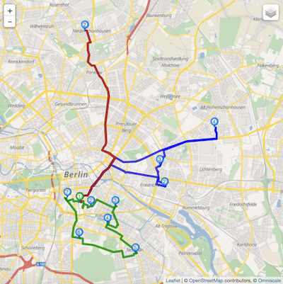
As you can see, 3 drivers are employed. This increases fixed employment costs as well as transportation costs. At the same time, however, it significantly reduces the completion time of the entire plan, i.e. of the last delivery. In other words, this optimization goal can be used to deliver more in less time. Wait, there are 4 drivers, why do I only see 3?
It is because the employment of a fourth driver cannot reduce the longest route anymore. But what if driver 4 got already paid? He needs to work! This brings me to the second option.
When using this objective, GraphHopper minimizes the longest route in terms of number of activities. It can be defined like this:
{ "objectives": [
    { "type": "min-max", "value": "activities" }
  ]
}
It results in a solution where all drivers are employed.
This is nice! Unfortunately, the forth driver (route marked in red) only has one activity now and by far the shortest route. Furthermore, the longest route from the last example (in terms of completion time) got even longer and got 2 new activities. In this example, it might be more favourable to keep this longest route as it was and distribute activities/stops evenly to all other routes. This can be achieved with the following optimization goal.
It combines the two optimization goals above and can be specified as easy as this:
{ "objectives": [
   { "type": "min-max", "value": "completion_time" },
   { "type": "min-max", "value": "activities" }
  ]
}
Applied to our example above, it yields the following solution.
This is a nice and balanced solution – at least when it comes to the specified indicators completion time and activities. Actually, there are various other indicators that requires your business to be balanced like unload time, tour length or demand. If you require other indicators than described here, please contact us.
If you want to try out our Route Optimization API or any other API such as Routing API, Map Matching API, Geocoding API, Isochrone API or our lightning fast Matrix API, register here and you get a free trial automatically.
Happy Routing!
We had the opportunity to improve two critical components of our Directions API.
The Matrix API is now up to 20 times faster for large matrices, which makes our Route Optimization API also significantly faster as it uses the Matrix API under the hood. You can find more details in our recent blog post.

The Geocoding API supports the new external provider “gisgraphy” and is currently the only alternative to the default provider that does not only support reverse geocoding but also autocomplete. Please read the documentation for a feature overview that also lists our other external providers like “nominatim” and “opencagedata“.
