Don’t hesitate to contact us:
Forum: discuss.graphhopper.com
Email: support@graphhopper.com
These are the three basic steps to solve a real world vehicle routing problem with GraphHopper’s Optimization API:
1) Assign geo locations to (road) network
2) Calculate travel times and distances
3) Solve vehicle routing problem
Each step impacts the solution of the vehicle routing problem. This article illustrates how 1) – the assignment of geo locations – affects solutions negatively, and how to mitigate these negative effects.
I would like to illustrate the problem with two simple examples. Let me start with the following traveling salesman problem. There is a single vehicle that needs to conduct 4 stops. This is our solution: The driver takes 41min and needs to travel 30km.
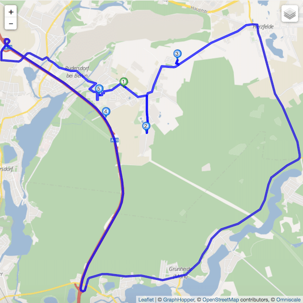
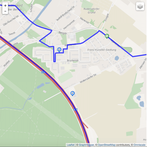
When looking at the map above the question arises why the driver needs to travel all the way over the motorway to get from stop 3 to 4 to 5. There is a simple reason for it. Stop 4 is assigned to the motorway, even though stop 4 should actually be assigned to the Woltersdorfer Street as illustrated below.
To better control the assignment at the level of the vehicle routing problem, we just introduced a new field to the address object called "street_hint". It can be used like this:
{
"id": "4",
"name": "serve sportpark",
"address": {
"location_id": "13.795629_52.460965",
"lon": 13.795629,
"lat": 52.460965,
"street_hint":"Woltersdorfer Straße"
}
}
This handy modification gives the snapping algorithm a hint to prefer a road link on the Woltersdorfer street rather than the motorway. This improves the solution of the above problem a lot. Now the driver only takes 25min and needs to travel 8km.
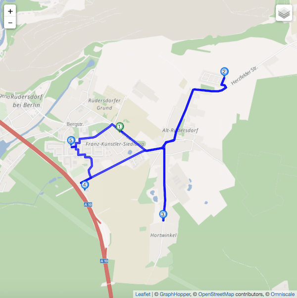
Note that if there is no road link belonging to Woltersdorfer street, the algorithm ignores the hint and proceeds as though as there were no hint, i.e. it assigns the closest road link. We also accept notation variations here.
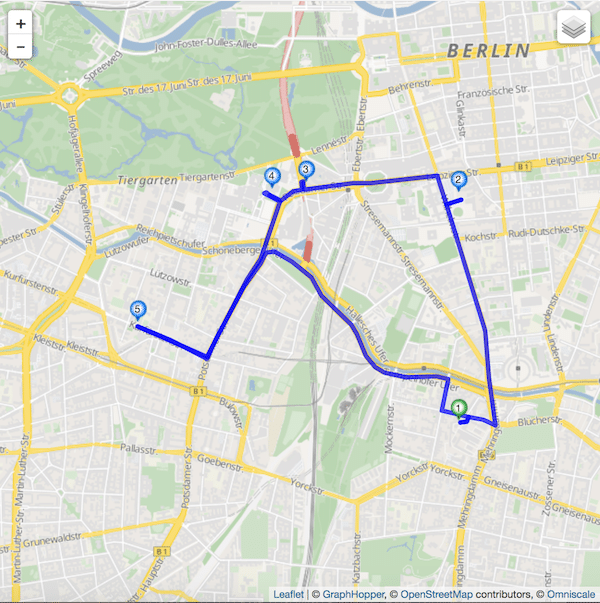
Let me show you another typical example from an inner city area in Berlin. It is again a simple traveling salesman problem with this solution:
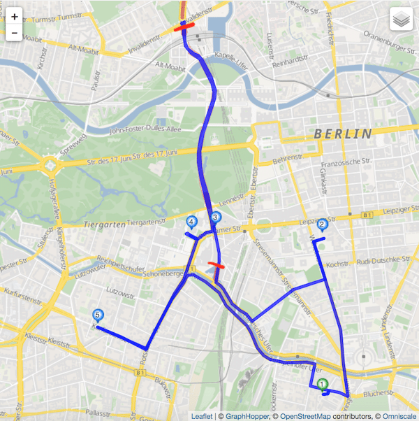
Why on earth does the driver need to travel this tail between stop 3 and 4? The reason is that there is tunnel going from the south red line to the north one, and the snapping algorithm assigns stop 3 to a tunnel link.
However, if this stop should not be located in the tunnel, but on the Ben-Gurion street above, we need to modify our address with “street_hint” as follows:
{
"id": "3",
"name": "deliver person on Ben-Gurion street",
"address": {
"location_id": "13.372159_52.509617",
"lon": 13.372159,
"lat": 52.509617,
"street_hint": "Ben-Gurion"
}
}
which yields the following solution:
Happy Routing!
In this post, we are going to look a bit into the future and analyse how the arrival of autonomous vehicles can reshape the existing transport systems and how fleet management systems can help us make the most of the new opportunities.
The idea of autonomous car have been inspiring people for many years, however, only quite recently automation achieved a level sufficient for autonomous vehicles (AVs) to hit the road. While AVs have not yet reached the level of full automation (Level 5, according to the SAE classification), in this post, we will focus on the operations of Level-5 AVs and specifically on robo-taxi (driverless taxi) services, which are aimed at providing convenient, safe, efficient and still affordable ways of travelling.
As a case study, we will take a city-wide replacement of private cars with robo-taxis in Berlin, Germany, a study carried out by the author of this post together with Joschka Bischoff and other researchers at TU Berlin (see references at the end of this post). We want to simulate a normal week day with one substantial difference: all trips usually made with private cars within the boundary of Berlin will now be served by robo-taxis. Altogether, this is more than 2.5 million trips with a significant afternoon rush hour peak when around 3:00 pm almost 100 taxi calls are made each second, which clearly reflects the size of the problem. The simulation was carried out in MATSim (Multi-Agent Transport Simulation).
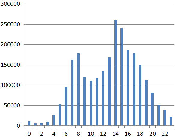
Hourly number of taxi calls shows a peak around 3 pm, which impacts the size of the robo-taxi fleet and poses a challenge to real-time taxi dispatch
To tackle this problem a fleet of 100,000 robo-taxis is dynamically dispatched by a real-time optimisation algorithm that reacts to incoming events, such as taxi calls or changes of vehicle location and status. While conventional taxis are typically dispatched according to the first-come-first-served (FCFS) rule, mainly because the taxi demand is relatively small, this strategy is not well suited when there is a lack of taxis. For the city-wide replacement of private cars with robo-taxis, we want to have a possibly smallest fleet that is able to operate efficiently under heavy load. In order to achieve that, we modified the dispatch strategy so that it follows the FCFS rule and sends the nearest idle taxi to the new customer only if there is at least one idle taxi (oversupply). However, if there are no idle taxis and at least one awaiting customer (undersupply) then whenever any taxi becomes idle, it is immediately dispatched to the nearest waiting customer. By doing this, we violate the FCFS rule, but at the same time we minimise the time spent on driving empty, which in turn increases the overall efficiency of the dispatch system.
The simulation was carried out for different fleet sizes, but we will focus on the scenario with 100,000 robo-taxis, which is a good compromise between the fleet size and quality of service as illustrated in the following two figures.
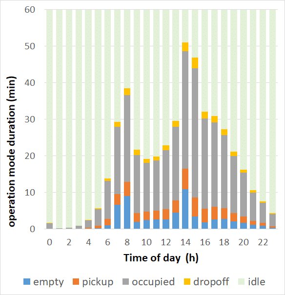
Hourly vehicle utilisation (empty – driving empty, pickup –picking up a passenger, occupied – driving with a passenger on board, dropoff – dropping off a passenger, idle – waiting)
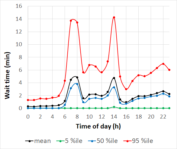
Passenger wait times over the day (mean, 5th percentile, median, 95th percentile)
With the exception of peak hours, robo-taxis are idle for most of the time. During the peak hour there is a substantial increase of empty drives, which is related to the scarcity of idle taxis. This impacts the wait time, which for some very unlucky passengers, can exceed 15 minutes, whereas the daily average is 2.5 minutes. However, the inconvenience of longer wait times can be mitigated by booking in advance.
All in all, the obtained results indicate that 1.1 million private cars could be replaced by 100,000 robo-taxis, which gives a replacement ratio of 1:11. However, fewer cars does not mean less traffic. Robo-taxis lead to a higher traffic volume due to empty mileage on drives between customers (the blue colour in the second chart), which is particularly high during peak hours. This significantly deteriorates the traffic conditions. In particular, traffic in the city centre is affected most, as illustrated on the following map showing differences in speed ratios (the ratio between the observed average speed and the maximum/free-flow speed on a link).
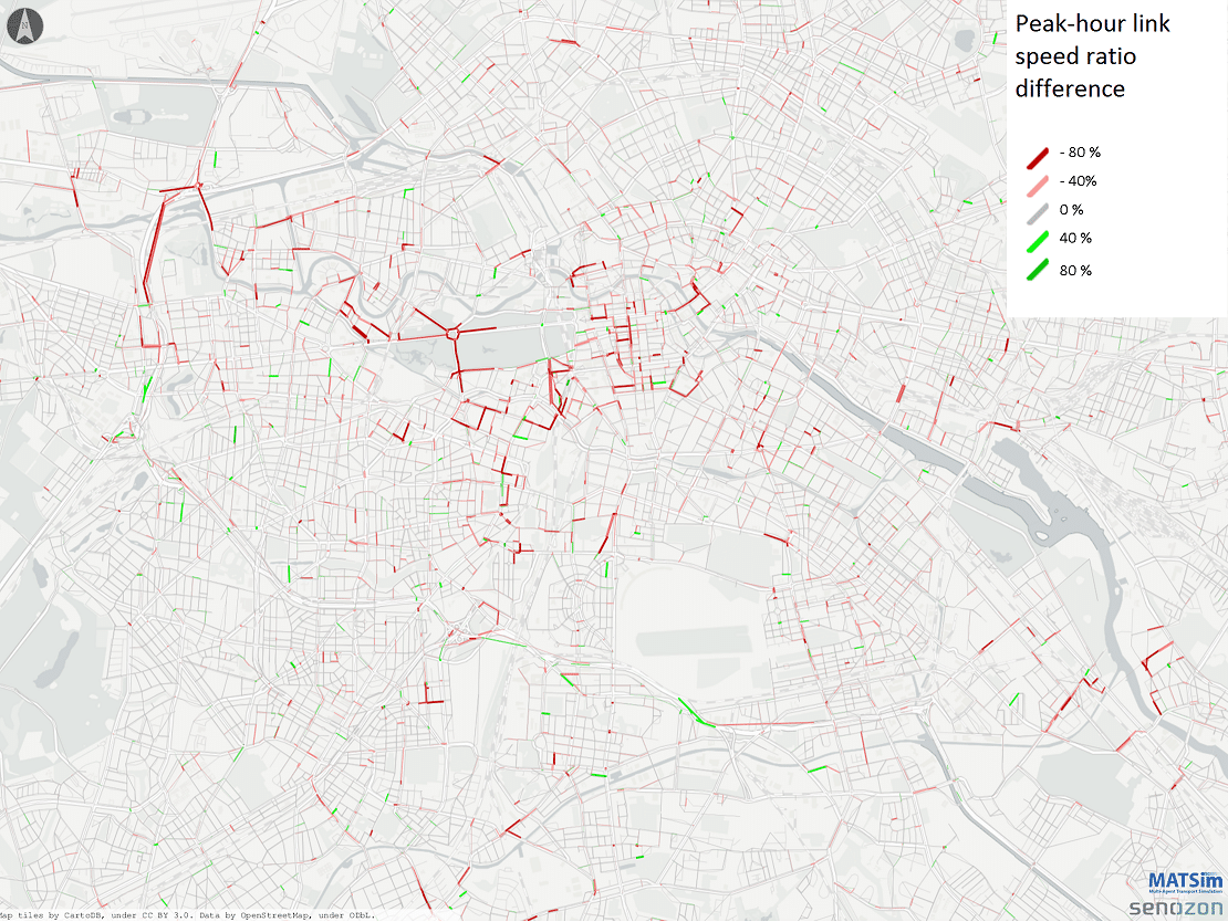
Differences in speed ratios before and after the introduction of robo-taxis during the afternoon peak hour. Interpretation: -40% for a link with a 50 km/h speed limit means that the average speed dropped by 20km/h after the introduction of robo-taxis.
Fortunately, autonomous vehicles are expected to move more smoothly in traffic, mostly due to shorter reaction times and hence reduced time gaps between vehicles. The current predictions estimate the road capacity increase at 1.5 to 2 (meaning the maximum flow could be 1.5 to 2 times higher). When we rerun the simulation taking into account even the less optimistic estimate of 1.5, it turns out that the introduction of robo-taxis significantly improves traffic conditions.
However, there is a risk that robo-taxis will generate a substantial additional travel demand, which may not be compensated by the predicted road capacity increase. This is where dynamic route optimisation may help us by extending the typical taxi service with additional features, such as sharing rides, relocating vehicles before traffic peaks or routing vehicles through such links that the impact on traffic is minimised.
As an example, let us rerun the robo-taxi simulation with the ride-sharing option and assume that up to 4 passengers may share a taxi at the same time and detours are allowed as long as the travel (wait + ride) time does not exceed 1.5 * t + 15 [min], where t is the direct (unshared) ride time from origin to destination. Whenever a new request arrives, the optimisation algorithm inserts the pickup and dropoff into the route of one of robo-taxis so that no constraint is violated (e.g. capacities or time windows) and the overall fleet operation time is minimised. By doing this, we try to maximise ride sharing and reduce the total mileage, which leads to reductions both of the fleet size and traffic volumes. As a result, we are now able to replace 1.1 million of passenger cars with a fleet of only 60,000 robo-taxis. The following chart illustrates the fleet-wide hourly ride sharing levels.
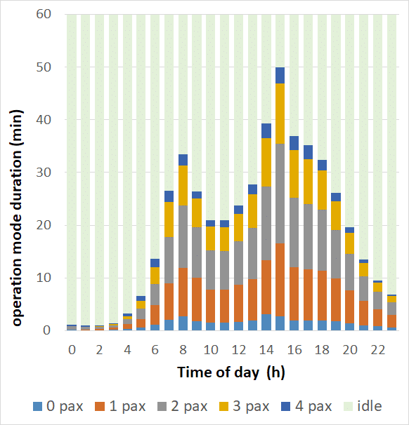
Hourly vehicle utilisation (0 to 4 pax – busy vehicles with 0 to 4 passengers on board, idle – waiting vehicles)
While the share of busy vehicles throughout the day looks similar in both cases (with and without ride-sharing), now we use only 60% of the original fleet to provide the service, which also means significantly less traffic (even less than in the base scenario with private cars). This makes the service more environmentally friendly and cost effective. Of course, from the traveller’s perspective, we have longer wait times (not a problem if trips are booked in advance) and ride times, but on the other hand, the reduced fare for shared trips may compensate for these inconveniences.
As we can see, one of the core elements of on-demand mobility is dynamic route optimisation and the way we dynamically route vehicles has a significant impact on the system efficiency. In particular, operating the future robo-taxi fleets will require application of real-time optimisation algorithms that immediately react to the high-flow streams of incoming events.
In the next posts, we will discuss new exciting challenges we face while developing such systems, and we will share with you a few words on the latest developments of Dynamic Route Optimization API.
More detailed information on the presented simulations:
These and related research papers can be found here.
More general information on autonomous vehicles and robo-taxis can be found on Wikipedia here and here.
