In our last blog post we elaborated the problem of finding a route through Dublin without passing by any Pub. Rory gave us the idea for this, and now again, pointed us to an article reporting that recently there was a Japanese man trying to visit each and every pub to drink a pint of Guinness.

From ‘avoid pubs’ to ‘visit all pubs’

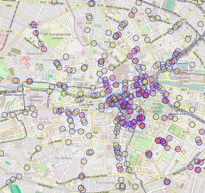
Thus, we were keen to see how the route looks if we reformulate the problem from “avoiding pubs” to a problem of “visiting all pubs”. It seems to be a similar problem just do the “inverse”, but it is not. This is the classical traveling salesman problem in contrary to a least cost path problem. The Japanese man called Abe used ‘The Dublin Pub Spotters Guide’ by Mac Maloney as pub guide. We do not have this guide. However, we retrieved 226 pubs located in the center of Dublin from OpenStreetMap via overpass. Additionally, we assumed that Abe started his journey at Connolly station, i.e. he walked all the way and stayed 30 minutes in every pub. Here is the problem on a map:

And what is the solution? To visit every pub exactly once he needs to walk 38 kilometers, i.e. approximately 7 hours and 46 minutes (neglecting the fact that the more beer he has, the slower he is able to walk from one pub to another). Considering that he stays in each pub 30 minutes, Abe’s pub project takes 5 days, 46 minutes in total.

How many days a more realistic pub journey will take?

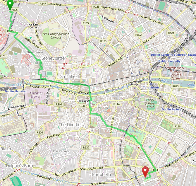
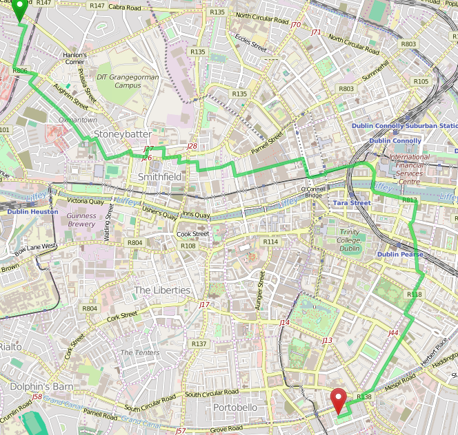
Apart from that making the Guinness project in four weeks is ambitious, visiting all pubs in a row is quite an additional challenge ;). Thus, to make it more realistic we reformulated the problem so that we give Abe some time to recover, i.e. we only give him 5 hours and 30 minutes time per day for his pub journey. Thus he needs to start at 6pm from Connolly station. By 11:30pm he needs to be back again. This is also in line with the opening hours of most of the pubs. The problem then turns into a vehicle routing problem with time restrictions where we not only want to find the best routes, but also to determine the number of days the pub project takes. Lets look at our solution. It takes 27 days to visit all pubs, 152 kilometers need to be walked corresponding to 1 day, 6 hours and 27 minute walking time. To illustrate this, look at the following figures showing the routes of day 1, 9 and 21. On the right side of each figure, one can see the highlighted route along with the pub locations marked in red. On the left side, there is a table showing the arrival and departure times for each pub as well as the cummulated distances.

These last pictures are from our route debugger, which is available in our dashboard and makes playing around with our API very simple. If you want to learn more, just visit GraphHopper.com and play with our live examples!

Discussion and comments happened at hackernews.

A long time ago there was a nice blog post

How to walk across Dublin without passing a pub

from Rory and there was even someone who tried this in real life. Now we thought how this would look like today using GraphHopper instead of the manual process described in the post.

It turns out that the whole process is much faster and simpler when using a routing engine. For people with little time you can grab the full sources here. First of all we need the data. Getting all pubs as Geojson today is very easy:

1. Go to Overpass Turbo
2. Go to the area of your choice, click on ‘wizard’ and enter ‘amenity=pub’
3. Click ‘export’ and ‘GeoJSON’

The data looks as follows:

Integrating the data in an open source routing engine like GraphHopper is also easy. Just look on how to create a custom weighting here. To avoid expensive operations while routing we convert the polygon or bounding box check into something fast like an ID check, only necessary for longer routes and probably not so much for this example. But we still do so as an example, by getting the nearest GraphHopper entry into the graph from the OSM data and all the surrounding edges via:

QueryResult qr = index.findClosest(lat, lon, EdgeFilter.ALL_EDGES);
EdgeIterator iter = explorer.setBaseNode(qr.getClosestNode());
while (iter.next()) {
  avoidEdgeIds.add(iter.getEdge());
}

Now we can use the set of ‘avoid IDs’ in the weighting method and increase the weighting appropriated:

public double calcWeight(EdgeIteratorState edgeState, boolean reverse, int prevOrNextEdgeId) {
  double w = super.calcWeight(edgeState, reverse, prevOrNextEdgeId);
  if (avoidEdgeIds.contains(edgeState.getEdge())) {
    return w * 1000;
  }
  return w;
}

The route with the normal “weighting=fastest” looks like:

Now, if you followed the installation instruction of the git repo (java, maven and git are required) then you can change the weighting=nopub e.g. in the URL then you’ll get a much longer route of 7.3km instead of 5.8km:

Conclusion

The whole center is today a no-go-area. And if you look closely it is even not fully possible to walk through Dublin and completely avoid alcohol and its results. The reason might be better OSM coverage for pubs or just more pubs. But the route only contains a reduced amount of pubs like the Abbey street. Such spots we could notify the user via special instructions, which could be a task for another blog post. Another task could be to persist the edge IDs to avoid importing the pub data on every start.

The first comment on the original blog post was “Good read! Next, can you create a route passing every pub!”. For the solution visit our talk about route optimization with GraphHopper in Berlin at the WhereCamp on 26th November and the solution is just one API call away…

The traveling salesman problem is the problem of finding the shortest possible route through a given set of locations whereby each loaction must only be visited once and the traveling saleman must return to its start location. A very good introduction into traveling salesman problems has been done by William Cook. It is fun to read!

One of the properties of the problem that makes it interesting and challenging at the same time is that the solution space, i.e. the number of possible routes, grows very fast with the number of locations to be visited. For example, for a 50 location problem there are 49! possible routes – when setting one location as start and end, and dealing with asymmetric travel distances. 49! results in a number with 63 digits.

Thus, for a certain number of locations visiting the entire solution space is no option anymore. However, mathematicians and operation researchers have developed methods that guarantee the optimal solution without visiting all possible routes, e.g. various branch and cut algorithms. Furthermore, they have developed methods that have been proven to find good solutions very fast, but cannot guarantee a certain quality. Latter are usually called heuristics.

Geoffrey de Smet recently wrote a nice article about “How good are human planners?”. He showed in a non-representative experiment that the ordinary heuristics humans apply to solve these problems are ok, but in comparison to machines they are not that good. Consequently, they can hardly judge the quality of algorithms that usually solve these problems much better than they can.

To judge the quality and speed of algorithms, scientists have developed artificial problems to benchmark them. These benchmarking problems usually come with a simple distance metric such as Euclidean distance, or with precompiled real world travel distances. This is the best way to evaluate the optimization algorithm. However, when solving real world problems, the computation time it takes to calculate travel times and distances based on real networks is relevant too. To put it in other words, point-to-point routing is an elementary part of solving these real world problems. Therefore, to benchmark the capabilities of our Optimization API to solve real world problems, we do two things here.

• First, to evaluate the quality of the applied optimization algorithm, we benchmark it against classical traveling salesman benchmarking problems.
• Second, we created 8 real world problems differing in the number of locations and measured the speed of solving the entire problem, i.e. not only the speed of solving the underlying optimization problem, but also the speed of assigning geo-codes to network links and solving the required point-to-point routing problems.

Classic Benchmark Problems

Lets start with benchmarking against the classical problems. Here we use a subset of problems from the TSPLib collected by the chair of discrete and combinatorial optimization at the Ruprecht-Karl-Universität Heidelberg. To keep it manageable, we only consider problems with up to 300 locations yielding 47 problems, solved them 3 times with a 2,2 GHz Intel Core i7 MacBook and averaged the results (to reduce random variations). The following table is an aggregated view on the results, i.e. we classified the problems according to their size (<25 locations, 50-100, 100-200 and 200-300) and averaged the computation time as well as the objective value relative to the best known solution.

[table id=1 /]

The table shows that in average our algorithm calculates best known results for problems smaller than 100 locations. For the residual problems it is shown that our results are not worse than 2 percent of the best known solution. Since these are average results, it is fair to also mention the worst result which is not worse than 5 percent relative to the best known result. The table also shows that the average computation time for a problem with a size smaller than 25 locations amounts to 23ms, whereas the computation time for a problem of size 50-100 locations amounts to 357ms.

Real World Problems

Lets conduct the second analysis. Here, we create 8 random real world problems of different size in the city of Berlin. That is we just draw 10, 25, 50, 100, 150, 200, 250 and 300 random geo codes in Berlin, and solved them with our Direction API. Again, we did that 3 times to reduce random effects and the impact of network delays. The following table shows the average computation time and the travel times determined by our Directions API. Note that computation time includes snapping geo-codes to OSM network, calculating n x n travel time matrix, optimizing the traveling salesman problem and network delays.

[table id=2 /]

Thus, it takes in average half a second to solve the entire problem with 25 locations, and 3 seconds to solve a problem with 100 locations. We think that this is rather fast. Thus, it allows us to solve several hundreds of these small to medium size problems on our servers in a minute. To give a visual impression of the solution for the 200-location problem, look at the following figure.

Note that we do not demand our Optimization API to produce optimal and best known results since this would be too expensive in terms of computation time. However, we want it to calculate very good and reasonable results in short time, and we designed our API such that it can deal with various additional side constraints without loosing much of its speed. Therefore, it cannot only be used to solve the classical traveling salesman problem, but also to solve problems where the salesman needs to consider time windows at locations, where he needs to consider his own legal rest periods, where he does not need to come back to its start location and where an arbitrary number of additional relations between locations exists (such as that location B needs to be visited directly after location A etc.).

Just play with our official live examples, sign up and get started!

Since several months we’ve been working on the Route Optimization API – a new part of the GraphHopper Directions API. And today it goes into beta status, i.e. we trust the software and our architecture enough that it can be used in production. Although it is used in production already we allowed us to change the API and even break it in certain areas which won’t happen anymore.

What is the Route Optimization API?

The Routing API solves the problem of finding routes between predefined locations where the order cannot change. Now the new Route Optimization API solves the heavier problem where the order of locations can be optimized. Furthermore, an arbitrary number of constraints like time windows, capacity restrictions of vehicles, driver skills and even driver breaks can be taken into account, and our API does not only allow solving single vehicle problems, but can consider multiple vehicles with multiple start and end locations. These problems are known as vehicle routing problem (where the traveling salesman problem is one problem type). Our Route Optimization API makes these complex problems easy to solve.

Traveling Salesman Problems (TSP)

In a later blog post we’ve covered the so called traveling salesman problem in more detail. For now here is a small example of a sightseeing tour through Berlin where randomly selected POIs were chosen: Checkpoint Charlie, the television tower, Berliner Ensemble, Berliner Dom and Staatsoper. One can define it as a simple routing request, with 3 via points and a fixed start and end point, and just needs to add the optimize parameter (optimize=true) to the Routing API. Look at the illustration below. It saves roughly 10% travel time (76min instead of 85min), and the more locations you have the bigger the savings can be.

 

Vehicle Routing Problems (VRP)

Furthermore, our Route Optimization API is able to solve vehicle routing problems with more than one vehicle,  i.e. real world scenarios happening everyday in supply chains of logistics. Therefore we’ve also added some more vehicle profiles including trucks to improve the estimated arrival time further. We will be covering this problem in more detail in a later blog post, but for now let us look at the following simple example:

Assume a fleet manager needs to dispatch 3 vehicles with start and end location at the main station. Each vehicle only has the capacity of serving 7 customers at maximum. In total, 20 customers that are randomly located in Berlin need to be served such that total transport time is minimized. This is a very prominent form of a vehicle routing problem, a capacitated vehicle routing problem. And the solution will then look like

This gives a first impression of what can be solved with our API. However, the problems one can actually solve with our API can be more complex e.g. minimize completion vs. transport time, minimize maximum makespan and many more interesting problems. Just play with our official live examples and customize them as they are open source. Sign up and get started!